Satellite-Based Data Assimilation System for the Initialization of Arctic Sea Ice Concentration and Thickness Using CICE5
[ad_1]
Introduction
Arctic sea ice is an important component of the Earth system in a warming climate that changes most dramatically during recent decades (Serreze et al., 2009; Screen and Simmonds, 2010; Perovich et al., 2017; Kwok, 2018). Arctic sea ice extent and thickness have consistently decreased rapidly in all seasons due to the anthropogenic forcing during last few decades (Kwok and Rothrock, 2009; Stroeve et al., 2012a). In addition to the contribution of anthropogenic forcing, internal variability dominating the Arctic summer circulation trend is also important cause of declining in September Arctic sea ice since 1979 (Ding et al., 2017). The rate of Arctic sea ice decline is unprecedented over at least the past 1,500 years according to reconstructed sea ice historical data (Kinnard et al., 2011), and an ice-free state is expected in the middle of twenty-first century according to climate model predictions under the high emission of the greenhouse gases (GHGs) scenarios (Wang and Overland, 2012; Notz and Stroeve, 2016; Guarino et al., 2020; Notz et al., 2020).
What is more, dramatic decrease of Arctic sea ice has increased interannual variability in the sea ice extent (SIE), particularly from summer to autumn. The interannual variability of the summer Arctic sea ice is non-linearly rising with a warmer climate, so that uncertainties for Arctic sea ice prediction also become large for recent decades (Goosse et al., 2009). Holland et al. (2008) showed the significant increase in standard deviation of September SIE anomaly in the global climate model projections, which eventually would contribute to decrease the predictability for Arctic sea ice in the future. On the other hand, Massonnet et al. (2018) suggested that Arctic sea ice volume will exhibit less year-to-year variability through the enhanced action of growth and melt processes as the ice thins in the future projections.
It has been recently recognized that Arctic sea ice plays an active role on the weather and climate system in the middle latitude in Northern Hemisphere as well as those in Arctic region (Zhang et al., 2012; Kim et al., 2014; Mori et al., 2014; Kug et al., 2015). The recent decrease in the sea ice affects the surface energy budget by the reducing the surface albedo and disappearing an insulating cap of the air-sea interfaces, which can increase the oceanic temperature to amplify the variation of the local near-surface temperature in Arctic (Stroeve et al., 2012b), then it induces the stationary Rossby wave-train to influence the climate in mid-latitudes particularly over the Eurasian and North America (Bader et al., 2011; Cohen et al., 2012; Mori et al., 2014; Kug et al., 2015), north Pacific such as the Aleutian low, and tropical central Pacific (Overland et al., 1999; Kennel and Yulaeva, 2020). That is, Arctic sea ice states are also considered as the cause of the weather and climate variability beyond the polar region (Deser et al., 2015). The possibility of mid-latitude effects of Arctic sea ice leads to increasing demand for the accurate predictions of the Arctic sea ice in recent decades, even though its influence on the mid-latitude climate significantly varies on the period analyzed, implying the necessity of the robust observational evidence (Overland et al., 2016; Blackport and Screen, 2020a,b; Cohen et al., 2020).
In addition, an accurate prediction of the Arctic sea ice leads to economic benefits by predicting the shipping route through the Arctic (i.e., Northern Sea Route, NSR) for commercial shipments between Europe/North America and Asia (Liu and Kronbak, 2010; Smith and Stephenson, 2013). Feasibility of the NSR is only possible when the climate model with high-resolution grid system is developed and the accurate predictions for the sea ice state (concentration and thickness) are guaranteed (Aksenov et al., 2017). Therefore, there has been a rising demand for Arctic sea ice predictions at sub-seasonal to interannual time scales (Eicken, 2013). In addition to the deterministic sea ice forecasts (Blanchard-Wrigglesworth et al., 2015; Wayand et al., 2019), as the forecast of Arctic sea ice is intrinsically uncertain due to the uncertainties originated from the chaotic nature of the sea ice component and irreducible model errors as with other climate system, probabilistic forecasts of Arctic sea ice have been explored recently to quantify the uncertainty in a forecast and to produce the optimal decision making (Dirkson et al., 2019; Gao et al., 2021).
The quality of Arctic sea ice prediction using the numerical model strongly depends on the degree of implementation of sea ice-related dynamical/physical processes in the dynamical model and the quality of the initial condition (Chevallier et al., 2013; Sigmond et al., 2013; Wang et al., 2013; Tietsche et al., 2014). In particular, Tietsche et al. (2014) insisted that shortage of the knowledge of Arctic sea ice initial conditions should impede the skillful predictions. To guarantee the skillful sea ice predictions, it is essential to improve the initial conditions by implementing data assimilation techniques using available observations (Lisæter et al., 2003).
Fortunately, the satellite-derived observational data of the sea ice concentration (SIC) have been successfully produced for over 30 years (Cavalieri et al., 1996). In addition, although retrieval methods are an early stage of development, pan-Arctic sea ice thickness (SIT) satellite observations have been produced since 2002 (Hendricks et al., 2018), and dataset with high spatial gridded resolution of 12.5 km and temporal resolution of 1 day have been also yielded from the 2010s (Tian-Kunze et al., 2014). Thus, several studies have carried out data assimilation of satellite-derived SIC and SIT into dynamical sea ice models using advanced assimilation techniques. Lisæter et al. (2003) used an ensemble Kalman filter (EnKF) to assimilate SIC data derived from Special Sensor Microwave/Imager (SSM/I) carried on board the satellites of the Defense Meteorological Satellite Program (DMSP). Lindsay and Zhang (2006) conducted a nudging scheme to assimilate observed monthly averaged SIC and sea ice velocity independently into the coupled ice-ocean model. Stark et al. (2008) assimilated the SSM/I SIC and sea ice drift data using an optimal interpolation scheme into the Met Office Forecasting Ocean Assimilation Model (FOAM). Caya et al. (2010) implemented the 3D-VAR to assimilate SIC into the Community Ice-Ocean Model (CIOM). The positive impact of assimilation on improving the simulation quality of the modeled SIC was well-established in aforementioned studies.
The next generation of researches emphasized the updates of the SIT in addition to the SIC for the accurate estimates of the growth/decaying speed of the sea ice, and the resultant sea ice openness regulating the ocean-atmosphere interactions are strongly dependent on the SIT. As a pioneer work, Tietsche et al. (2013) and Massonnet et al. (2013, 2015) showed that the quality of SIT in their reanalysis is improved by updating both SIC and SIT with the given SIC increment (i.e., multivariate updates). However, Massonnet et al. (2015) discussed that those results are needed to be further verified because of the inadequate observations of SIT and have large uncertainties in the estimation of SIT. In addition, their methodology has a clear limitation to improve the SIT simulation as the SIT updates is solely dependent on the SIC observation, and the degree of the update is based on the modeled relationship between SIC and SIT.
There are attempts directly assimilating SIT using satellites-based SIT observation (Yang et al., 2014; Chen et al., 2017; Blockley and Andrew Peterson, 2018; Mu et al., 2018; Xie et al., 2018). For example, Yang et al. (2014) shows that the data assimilation of SIT observation of SMOS into an ocean-sea ice model using local ensemble singular evolutive interpolated Kalman filter (SEIK) improves the forecast skill of SIT. Xie et al. (2018) assimilated SIT observation of merged measurements from CS2 and SMOS (CS2SMOS) into the TOPAZ4 system with Deterministic EnKF during boreal winter and showed the improvement in the SIC and sea ice drift in the central Arctic Ocean and Kara Sea.
However, the period of the experiments for the SIT assimilation is only for few months or years in previous researches, therefore, it was rather short to assess the degree of improvement in simulating long-term climatology and the interannual variability (Massonnet et al., 2015). This is, it has not been tried to reconstruct the Arctic sea ice states more than a decade by assimilating both satellite-based SIC and SIT observations.
In this study, we reconstructed the Arctic sea ice states for a decade (i.e., during 2010–2019) by assimilating satellite-derived SIC and SIT into the Los-Alamos sea ice model version 5.1.2 (CICE5) using Ensemble Optimal Interpolation (EnOI) scheme (Backeberg et al., 2014; Mignac et al., 2015; Kaurkin et al., 2016). In addition, the reanalysis quality by assimilating SIC observation is evaluated through the data assimilation experiment for two decades (i.e., during 2000–2019). This article is organized as follows. The description of the model and methods is given in Section Data and Methods. In Section Results, the impact of the data assimilation on the SIC and SIT states are assessed. Summary and Discussions are given in Section Summary and Discussions.
Data and Methods
The Sea Ice Model and Atmospheric/Oceanic Forcing
We used the Community Ice CodE (CICE) version 5.1.2 sea ice model, will be referred as CICE5 for simplicity, developed by the Los Alamos National Laboratory (LANL) (Hunke et al., 2015). The CICE model is a state-of-the-art sea ice model, which is originally developed as a stand-alone version, and it is now set up as a sea ice component of the National Center for Atmospheric Research (NCAR) Community Earth System Model (CESM) (Gent et al., 2011; Hurrell et al., 2013; Danabasoglu et al., 2020), and the others (Maclachlan et al., 2015). The CICE5 is a multicategory sea ice model to describe the ice thickness distribution with five thickness categories (fixed thickness boundaries are 0, 0.64, 1.39, 2.47, and 4.57 m by default). The sea ice in each category consists of seven vertical layers and one snow layer to resolve the sea ice temperature and salinity variations. The CICE5 has a thermodynamic process of mushy layer thermodynamics and a dynamic process of elastic-anistropic-plastic dynamics (Wilchinsky and Feltham, 2006; Turner et al., 2013). The most complex physics parameterization schemes such as melt pond and ridging is recently added in this version of the CICE. The horizontal resolution of this model is 1° approximately with 320 × 384 dimensions on a displaced pole grid and the time step is 1 h.
In this study, CICE5 is forced at the surface with atmospheric and oceanic fields. The National Center for Environmental Prediction Reanalysis 2 (NCEP R2) dataset is used for atmospheric forcing (Kanamitsu et al., 2002). The atmospheric forcing for CICE5 was passed on to the sea ice in flux form at the atmosphere-sea ice boundary (Lee et al., 2019). The near-surface atmospheric variables [6-hourly specific humidity (kg kg−1), 2-m air temperature (K), 10-m U-wind and V-wind (m s−1)] was used to calculate the turbulent fluxes using bulk formulae (Large and Yeager, 2009), and the near-surface air density (kg m−3) was calculated using the relationship delineated in Large and Yeager (2009). Monthly mean downward shortwave/longwave radiation (W m−2) and total precipitation rate (kg m−2 s−1) were used as atmospheric forcing.
The Optimal Interpolation Sea Surface Temperature (OISST) version 2 from National Oceanic and Atmospheric Administration (NOAA) (Reynolds et al., 2002) was used for daily sea surface temperature (SST) () forcing. The SST of mixed-layer slab ocean model in CICE5 is nudged toward the OISST data with 21-day Newtonian relaxation time-scale. The sea surface salinity was fixed constant value of 34 psu in this work.
Data for Assimilation and Validation
The satellite-observed daily SIC are obtained from the National Snow and Ice Data Center (NSIDC, http://nsidc.org/data/NSIDC-0079). They are derived from the Scanning Multichannel Microwave Radiometer on the Nimbus-7 satellite and from the Special Sensor Microwave Imager/Sounder (SSMIS) aboard Defense Meteorological Satellite (DMSP) F17 using the bootstrap algorithm (BT) version 3 (Comiso, 2017). The SSMIS BT data is on the polar stereographic projection with a spatial resolution of 25 km. The observational error value of 0.15 is uniformly given for accounting for measurement and representation errors (Janji et al., 2018), according to suggestion of Tonboe and Nielsen (2010). The OISST version 2 reanalysis data for daily SIC is also used for constraining the long-term control simulations to obtain the stationary ensemble perturbations as explained in Section Data Assimilation Scheme (Reynolds et al., 2002).
For SIT, the satellite-observation data have been derived from two different dataset of CryoSat-2 (CS2) and Soil Moisture Ocean Salinity (SMOS). The CS2 SIT is used here (http://nsidc.org/data/RDEFT4). The CS2, the European Space Agency (ESA) satellite mission, Level-4 SIT data based on radar altimeter measurements of sea ice freeboard is used for the area where the SIC is >0.7 (i.e., 70% of total area in the corresponding grid point) (Kurtz et al., 2014; Kurtz and Harbeck, 2017). The period for CS2 assimilation spans from January 1, 2011 to December 31, 2019. The SMOS is obtained from (https://icdc.cen.uni-hamburg.de/thredds/catalog/ftpthredds/smos_sea_ice_thickness/catalog.html). The L3C SMOS, the ESA mission, version 3.1 from January 1, 2011 to April 15, 2018 and version 3.2 from October 1, 2018 to December 31, 2019. Daily thickness data derived from L3B brightness temperatures using a single layer emissivity model is used for assimilating the modeled sea ice thinner than 1.0 m (Kaleschke et al., 2012, 2016; Tian-Kunze et al., 2014). The CS2 data is on the polar-stereographic grid system with a horizontal resolution of 25 km, and the SMOS data is on the NSIDC polar-stereographic grid system with a horizontal resolution of 12.5 km. The uncertainties of the observed SIT data are 1.5 m (0.3 m for random and + 1.2 m for systematic) for CS2 and 0.7 m (averaged of thin thickness) for SMOS, according to Chen et al. (2017). The satellite-based SIT observations are only available in the cold season from September (October) to May (April) for CS2 (SMOS and CS2SMOS), as it is difficult to discriminate between measurements from open ocean and sea ice due to melt ponds forming on the sea ice surface during the melt season (Tilling et al., 2018).
The verification for the quality of updated sea ice field by assimilating satellite data is conducted by utilizing observation and reanalysis data. The daily SIC derived from passive microwave sensor data (SSM/I) using the NASA Team algorithm (NT) is used to validate the reanalysis output (Cavalieri et al., 1996). The SSMIS NT data is used here (http://nsidc.org/data/NSIDC-0051). The Pan-Arctic Ice-Ocean Modeling and Assimilation System (PIOMAS) SIC and SIT are also used (Zhang and Rothrock, 2003). The weekly averaged SIT product version 2.3 of CS2SMOS derived from merging CS2 and SMOS using an optimal interpolation scheme is used to validate the updated thickness field (Ricker et al., 2017). The CS2SMOS data is used here (http://spaces.awi.de/display/CS2SMOS). Since CS2SMOS is created by merging CS2 and SMOS, there is some overlap with the assimilated data set. The grids of CS2SMOS are projected onto the 25 km EASE2 Grid. The model output, observation and reanalysis data are all re-gridded onto the 1 rectilinear latitude/longitude grid system from a displaced pole grid system used to solve the polar singularity problem for model and from Polar-Stereo graphic for satellite observations.
Data Assimilation Scheme
The satellite-derived sea ice data is assimilated using an Ensemble Optimal Interpolation (EnOI) scheme (Figure 1). The EnOI method approximates the background error covariance matrix (B matrix) by using a stationary ensemble member instead of a multiple realization of the model for the Ensemble Kalman Filter (EnKF; Evensen, 2003). Note that, because the mean state of Arctic sea ice is changing rapidly, the EnOI method with stationary B matrix used in this study has a limitation that it would cause a performance degradation compared to techniques considering flow-dependent features such as EnKF. While the EnKF is advantageous by using state-dependent ensemble perturbations, the use of EnKF is often limited as it requires multiple numbers of realization. Therefore, the EnOI is a cost-effective alternative to the EnKF to assimilating the complex dynamic models requiring high computation costs to operate (Oke et al., 2007). As a result, the data assimilation algorithms based on the stationary B matrix is still widely used to produce many SIC reanalysis products such as HadISST with OI (Rayner et al., 2003), NOAA OIv2 with OI (Reynolds et al., 2002), and ECMWF ORAS5 with 3D-Var (Zuo et al., 2019).
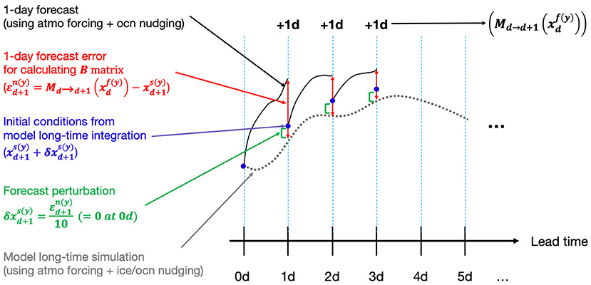
Figure 1. The schematic of the generation system for forecast error perturbations of for calculating stationary background error covariance matrix (i.e., B matrix). The black (dotted) line represents the model long-time simulation nudged sea ice and ocean reanalysis with atmospheric forcing and the black (solid) line represents the 1-day forecast experiments forced atmospheric forcing data without restoring sea ice fields. The blue dot represents the initial conditions from the model long-time simulation. The red bidirectional arrow represents the 1-day forecast errors and the green left bracket represents the forecast perturbations using the bred vectors.
In our work, to obtain the stationary ensemble perturbations, two sets of model integrations are performed. First, long-term control simulations are obtained by nudging the daily OISST sea surface temperature (SST) data along with the daily OISIC SIC, and monthly PIOMAS SIT data (dotted black line in Figure 1). The restoring time scale are 21-day for SST, 6-h for SIC, and 5-day for SIT. Note that the small change in the nudging time-scale does not lead systematic changes in the nudged states. The state vector in a control simulation is denoted as , where d is dth day of a year, and y denotes a year between 1982 and 2019.
Secondly, the perturbed experiment is performed to obtain the ensemble perturbations , which is the perturbation for the stationary B matrix. Initially (i.e., at January 1st, 1982), the initial condition by adding a random perturbation to a control simulation (i.e., ) are generated. Then, 1-day forecasted state is obtained by integration the model for 1-day [i.e., , where Md→d+1 is the dynamical forecast model from day d to d+1]. Then, the difference from the control simulation at a corresponding day (i.e., ) is defined as the perturbation (red bidirectional arrow in Figure 1). This difference is rescaled by 10% of its original amplitude, then, added to the initial condition at next day (i.e., ) (Green left bracket in Figure 1). This procedure is repeated for every day from 1982 to 2019 to obtain the . As a result, the procedure to obtain the perturbations is similar to those for bred vectors (Toth and Kalnay, 1993, 1997).
The reason to utilize the bred vector approach is to prescribe fast-growing perturbations that can successfully mimics the forecast errors (Toth and Kalnay, 1997). The fast-growing errors dominate total forecast errors by definition, while the contribution of the non- or slow-growing errors for total forecast error becomes smaller in time. Therefore, the bred vector, which is known as a fastest growing perturbation, effectively represents forecast uncertainty with limited the number of ensemble members. Since the number of ensembles (38 in this study) is limited compared to the degrees of freedom of the model (about 105 of CICE5), the ensemble perturbations generated by the procedure mimicking the breeding method grows faster than others to better represent total forecast errors with the limited number of samples.
The procedure for generating B(d) matrix (d denotes a number of day varying from 1 for 1st January to 365 for 31th December) using the perturbations is as follows. B(d) matrix has size of Nb × Nb (Nb is a dimension of the state vector) and denote the forecast error state vectors at day d in year y with size of Nb × 1. By assigning each year’s perturbation sequentially at each column, εd for day d is generated whose size is Nb × Ny, where Ny is the number of years (i.e., 38). The stationary B(d) matrix is constructed as . As B matrix is separately formulated by the calendar day, the B matrix accounts to the seasonal spatial differences in the perturbations. The B matrix for the each variable is formulated separately in a univariate sense: the observed information of one variable had no effect on the others during the assimilation procedures.
It should be noted that the generating algorithm of ensemble error perturbation used in this study does not take into account the model uncertainty originated from the physical parameters or the boundary conditions. That is, only the uncertainty led by the instability in the system was considered in the background error covariance matrix B, which can underestimate the amplitude of the error in the background states.
Then, in order to prevent non-physical update of analysis by the observation at unrealistically remote region, the localization scheme of Local Analysis (LA) is carried out (Sakov and Bertino, 2011). A localization radius of 800 km is applied as in Kimmritz et al. (2018) and Massonnet et al. (2015). With LA, the updates at each grid point are applied using observations within a specified distance. In addition to this, LA uses a quasi-Gaussian weight function as a localization function (Gaspari and Cohn, 1999), so observation and background error covariance in observation space are downweighted with increasing distance from the updated grid point like a Localized Ensemble Transform Kalman Filter (LETKF) (Hunt et al., 2007). Post-processing to conserve physical ranges for such variables is applied to keep the analysis states as physically reasonable values. That is, in the case with analysis value of the SIC with negative, and value >1, they are changed to 0, and 1, respectively (Kimmritz et al., 2018). The minimum value of the SIT analysis is set to 0.
In this study, the CICE5 has five categories of the SIT. A fractional sea ice area of each category is a prognostic variable, however, the total SIC, which is denoted by the sum of fractional ice areas for each category, is a diagnostic variable. As the satellite-derived SIC data only provide the aggregated concentration, the SIC increment is calculated using the difference between the modeled total SIC and the observed SIC. Then, analysis increment of total SIC are distributed to each category according to the modeled percentage of the SIC in each category with respect to the total value as method used in Chen et al. (2017). Each category of the SIT is also updated in the same way. Although the EnOI also can facilitate the multivariate scheme as in Zhang et al. (2018) to update each SIT category, it has not been validated whether the static covariance matrix between the aggregated SIT and SIT in each category successfully operates for the multi decades. For this reason, we adopted a relatively simple scheme as aforementioned.
When the SIC increment is positive in the case of both SIC and SIT is 0, the SIC in each category is updated by multiplying the pre-defined ratio for each category. The pre-defined ratios are 60, 20, 10, 5, and 5%, for the category 1–5, respectively. The SIT in each category is updated as a averaged value of the upper and lower thickness limit of each category, which is 0.32, 1.02, 1.93, 3.52, and 6.95 m for the category 1–5, respectively. To update the positive SIT increment in the case of both SIC and SIT is 0, the SIT in each category is updated by multiplying the aforementioned pre-defined ratios, and the SIC in each category is updated by dividing the SIT increment to the aforementioned fixed SIT values.
Experimental Design
The impact of data assimilation of the SIC and SIT is investigated by comparing the quality of the reanalysis in three experiments. “noDA” is a control experiment forced by atmospheric and oceanic forcing fields without any data assimilation. It should be noted that the noDA experiment is not same as long-term control simulation used to obtain the ensemble perturbations in Section Data Assimilation Scheme. The long-term control simulation used to generate ensemble perturbations is the experiment in which sea ice fields are nudged in addition to atmospheric and oceanic forcing, but noDA is driven by forcing only without nudging of sea ice. “Ver1” is an experiment assimilated only SIC, and “Ver2” assimilates both SIC and SIT satellite data. In Ver2, the state vectors for SIC and SIT are constructed and updated separately. The period for the data assimilation in Ver1 is 2000–2019. The data assimilation of the SIT in Ver2 was performed from 2011 to 2019 when SIT observation data is available. Therefore, the reanalysis value before 2011 for Ver2 is identical to Ver1. All data assimilation experiments have a spin-up time of 1-year.
Results
Properties of the Background Error Covariance Matrix
Figure 2 shows the standard deviation (STD) of the SIC perturbation for calculating B matrix at 15th January, April, July, and October. In January, the STD of SIC perturbation is relatively high in the marginal sea ice regions, while it is quite small over the rest of areas including the North Pole (Figure 2A). This denotes that the instability leading the growth of the SIC is relatively high over the marginal sea ice regions including the Atlantic sector of the Barents and Greenland Seas and in the Pacific sector of the Bering Sea and Sea of Okhotsk, and these regions are characterized by strong atmospheric and oceanic variability during boreal winter (Semenov et al., 2015). In April, the overall STD pattern is similar to January, but the amplitude is relatively weak (Figure 2B). The SIC variability in July and October shows a reduced regional difference compared to boreal winter and spring season (Figures 2C,D). These features are evident by the year-to-year variability shown in satellite observations for the same period (not shown). This implies that the background error perturbations would reflect the inter-annual variability of the sea ice in observation and the state-of-the-art numerical models.
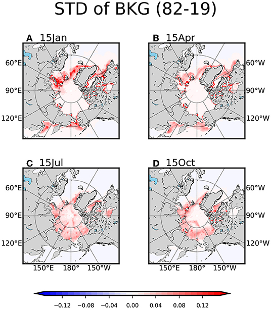
Figure 2. The year-to-year standard deviation at 15th January (A), April (B), July (C), and October (D) of forecast error perturbations for sea ice concentration (a fraction from 0 to 1) generated by using long-time integration during 1982–2019.
To examine the detailed spatial distribution of the B matrix, Figures 3A,D shows the global covariance patterns of the background error perturbations with respect to two selected points at 15th February, and October, respectively. Note that the localized covariance pattern is shown as in a final form of B matrix for the data assimilation. The covariance pattern with respect to the East Greenland (75°N, 10°W) is tilted in northeast-southwest direction (Figure 3A). This tilted spatial distribution is similarly shown in the SIC and sea surface temperature (SST) regression patterns using monthly anomalies from long-term simulation (i.e., noDA) (Figure 3B). More importantly, the tilted direction of the covariance pattern is consistent with the direction of the climatological sea ice drift, indicating that the East Greenland Current (EGC) is a major contributor to transport sea ice export southward along the continental margin (Figure 3C). This indicates that the sea ice particle mainly moves southwestward, therefore, the covariance with respect to any given point around this region would have relatively high values in southwest direction.
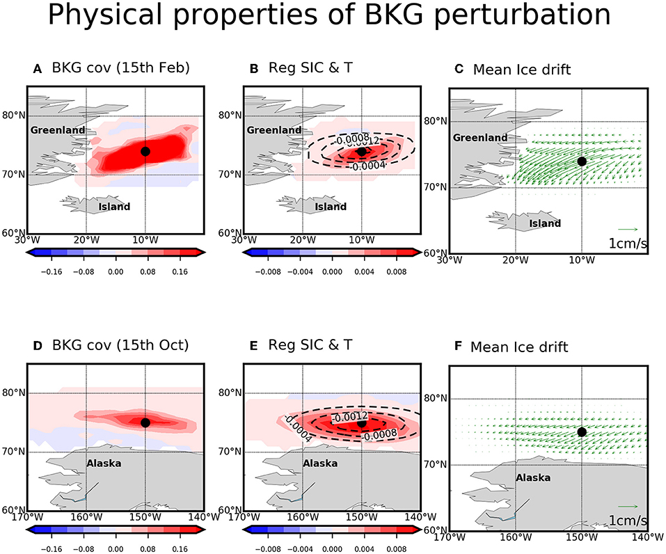
Figure 3. The covariance patterns (A,D) in forecast error perturbations of sea ice concentration (a fraction from 0 to 1) generated by using long-time integration, the regression patterns [shaded for sea ice concentration and contour for sea surface temperature (°C); B,E], and mean sea ice drift (cm/s; C,F) in model long-time integration outputs during 1982–2019. The covariance and regression patterns between a selected grid point (A–C: 75N, 10W in Greenland Sea; D–F: 75N, 150W in Beaufort Sea) and global grid points are left and middle column. The upper (lower) panels are results at 15th February (October). All the plots are localized using quasi-Gaussian weight function with localization radius of 800 km.
Similarly, over Beaufort Sea (i.e., 75°N, 150°W), the covariance pattern exhibits zonally-elongated pattern (Figure 3D), and it is also shown in the regression using monthly SST and SIC from long-term simulation (Figure 3E). The Beaufort Gyre (BG), which flows westward, can be responsible for this zonally-elongated pattern by transporting sea ice particle along the BG. This clearly demonstrates that the perturbations for the B matrix reflect the physical properties and balances associated with the sea ice variability.
Figure 4 shows that the time evolution of SIC anomalies over 2000–2019 at the two points used in Figure 3 for the observation and background state of Ver1 and Ver2. The amplitude of the STD of the ensemble perturbations, used to formulate B matrix, are added to, and subtracted from the background state (i.e., before update by assimilation). The observations are generally within the uncertainty range of the model states estimated using stationary ensemble perturbations. It can be also seen that it is also well-represented when zooming in on 2007 (Figures 4B,D). This indicates that the amplitude of B matrix properly measures the amplitude of the model uncertainty to some extent.
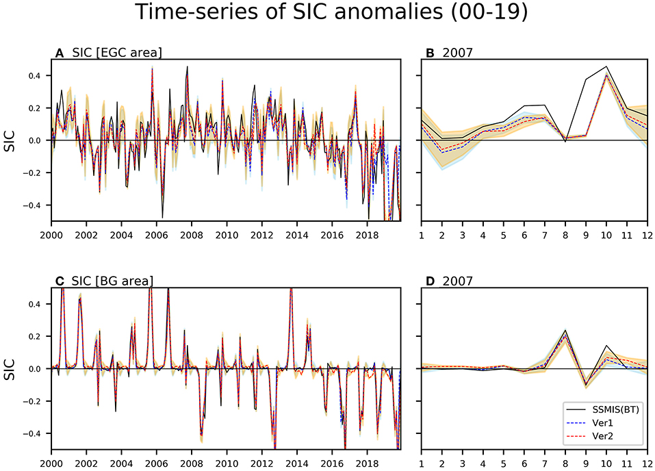
Figure 4. The temporal evolution over 2000–2019 (A,C) and in 2007 (B,D) of sea ice concentration anomalies (a fraction from 0 to 1) for observation (black) and background states of Ver1 (blue) and Ver2 (red) at a grid point used in Figure 3 (A,B: 75°N, 10°W in East Greenland Current area; C,D: 75°N, 150°W in Beaufort Gyre area). The orange (skyblue) shading marks the uncertainty (standard deviation) of the ensemble perturbations.
The Effect of Data Assimilation
Climatology and Seasonal Cycle
Figure 5 shows that the climatological seasonal cycle of sea ice extent (SIE, the summed area of all Arctic grid points with SIC > 0.15) over 2000–2019 (Figure 5A), and 2011–2019 (Figure 5B). The STD of the analysis errors representing the uncertainty embedded in the final reanalysis product (Xa) is obtained by calculating the diagonal component of the equation , where Pa, Pb, and R are the covariance matrices of the analysis, background, and observation, respectively, and H is observational operator.
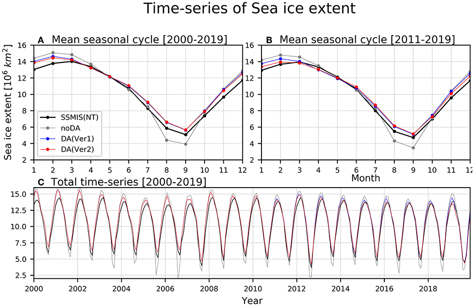
Figure 5. The mean seasonal cycle of Arctic sea ice extent index (106km2) during 2000–2019 (A) and during 2011–2019 (B) and temporal evolution over 2000–2019 (C) for SSMIS NT satellite data (black), noDA experiment (gray), Ver1 (blue), and Ver2 (red). The orange shading marks the uncertainty (standard deviation) of the analysis.
Compared to noDA, the seasonal evolution of the SIE in Ver1 and Ver2 becomes quite similar to the satellite observation (i.e., SSMIS NT). For example, in Ver1, the SIE is almost identical to the observation, and exhibited a relatively small difference only from November to February. On the other hand, in noDA, the SIE tends to be systematically underestimated, and overestimated during melting, and freezing season, respectively. The negative SIE bias in noDA during the boreal summer is due to the excessive bottom melting process during previous seasons (not shown). Then, the ice thinning during boreal summer play a role on the increase in the sea ice production during the ice growing season, which may contribute to the excessive SIE during boreal winter (Massonnet et al., 2018). The reduction in the climatological SIE bias in the Ver1 and Ver2 compared to the noDA is particularly robust in August and September, which is a melting season, rather than during January and February, which is the ice freezing season. This improvement in simulating SIE in Ver1 and Ver2 is also clearly shown in monthly time-series (Figure 5C).
It is interesting to note that the SIE in Ver2 is better than that in Ver1, indicating that the assimilation of the SIT observation in Ver2 further reduces the climatological bias in SIC in Ver1 (Fritzner et al., 2019). The SIE in Ver2 exhibits smaller climatological bias during January-February than that in Ver1. The improvement is minimal during 2000–2019, however, it becomes clear during 2011–2019 (Figures 5B,C). On the other hand, SIE in Ver2 is almost identical to that in Ver1 during boreal summer. This might be due to the fact that the SIC is already well-fitted to the observed by assimilating the SIC during boreal summer.
Figure 6 shows the spatial distribution of the climatological SIC of SSMIS NT and bias in noDA and Ver1 in February and August when the improvement in the SIE simulation was robust. The observation shows that the sea ice is distributed not only in polar regions but also in the subpolar regions such as Sea of Okhotsk, Bering Sea, Labrador Sea, and Baffin Bay in February (Figure 6A). The subpolar regions have no sea ice in August (Figure 6D). The climatological bias of SIC in noDA is greater than the observation about 0.3 in most of marginal ice zones, while it is relatively weak over polar region (Figure 6B). The positive bias of SIC in the noDA in most of marginal areas is significantly reduced more than a quarter in Ver1 (Figure 6C). In August, the negative bias of SIC in noDA reached up to −0.4 throughout the central Arctic Ocean with relatively weaker bias amplitude over Canadian Archipelago (CAP) region (Figure 6E). This negative bias is almost disappeared in Ver1 (Figure 6F). This confirms that the SIC data assimilation improves climatological state of the assimilated variable in both freezing and melting seasons.
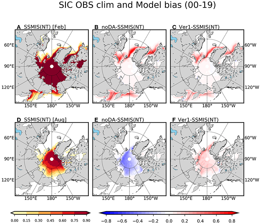
Figure 6. The climatology of sea ice concentration (a fraction from 0 to 1) of SSMIS NT satellite data (A,D) and climatological bias in noDA (B,E) and in Ver1 (C,F) with respect to the satellite observation in February (A–C) and August (D–F) during 2000–2019.
To examine the simulation quality of the climatological SIT, Figures 7A,B show the Northern Hemisphere-averaged monthly SIT climatology, and the spatial distribution of the climatological SIT of CS2SMOS and bias in Ver1 and Ver2 in February. Note that only the calendar months when satellite SIT observation is available are drawn. Over the thin SIT area (SIT of SMOS < 1 m), the SMOS SIT is kept as a nearly constant value (i.e., 0.4 m) from November to March (Figure 7A), possibly due to the cancellation between the SIT thickening of the pre-existing sea ice and the SIT reduction by the new formation of the thin sea ice during freezing season. This constant SIT climatology from November to March is not successfully simulated in noDA, implying that the new sea ice formation is weakly simulated in the model. On the other hand, the SIT climatology is kept as the constant in Ver1. However, the positive SIT bias about 0.2 m is shown throughout all seasons in Ver1. The SIT bias in Ver2 is systematically reduced compared to that in Ver1, while keeping the constant SIT climatology from November to March. This indicates that the simulation quality of the SIT climatology is improved by the direct injection of the SIT observation.
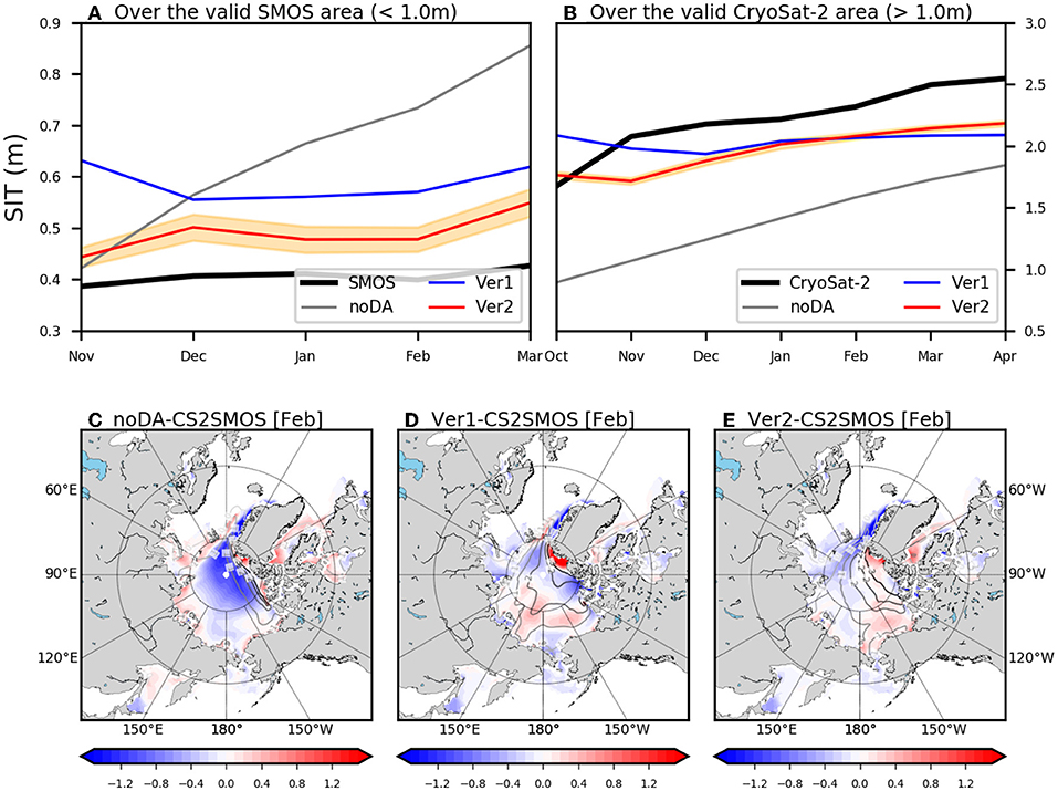
Figure 7. The mean seasonal cycle of sea ice thickness (m) averaged over the valid SMOS area (A) and over the valid CryoSat-2 area (B) during 2011–2019 for satellite observation used for assimilation (black), noDA experiment (gray), Ver1 (blue), and Ver2 (red). The orange shading in (A,B) marks the uncertainty (standard deviation) of the analysis. The climatological bias in noDA (C), Ver1 (D), and Ver2 (E) with respect to CS2SMOS in February. The contour lines in (C–E) represent the climatology in each model experiment.
Over the thick SIT area (SIT of CS2 > 1 m), the monthly CS2 climatology is increasing from October to April as it is the freezing season (Figure 7B). The new sea ice formation in those regions is not robust as it is already filled with the sea ice from the beginning of the freezing season. Even though the increasing trend from October to April is shown in noDA, the negative SIT bias is overwhelmed for all seasons. In Ver1, the negative SIT bias is significantly decreased, however, the thickening of SIT during the freezing season is not simulated. For example, the climatological SIT in CS2 is increased from about 1.7 m in October to 2.5 m in April, while that in Ver1 is continuously about 2 m from October to April. On the other hand, in Ver2, the negative SIT bias is reduced by keeping the increasing trend during the freezing season to some extent.
The spatial distribution of the climatological SIT bias in February also demonstrates the positive impact of the SIT data assimilation in Ver2 (Figures 7C–E). The strong negative bias of SIT in noDA is distributed in central Arctic ocean (Figure 7C). The climatological SIT in CS2SMOS exhibited a maximum value over the CAP region (not shown), and this spatial feature is well-simulated in both experiments to some extent (contours in Figures 7D,E). As a result, the SIT bias in both Ver1 and Ver2 is not robust over the CAP region (shadings in Figures 7D,E). In more detail, the amplitude of the SIT bias in Ver2 is <0.5 m over the CAP region, while that is reached up to 1 m in Ver1, supporting the notion that the SIT bias is systematically reduced through the assimilation of the observed SIT data.
The next question is whether the realistic SIT simulation by assimilating SIT observation contribute to improve the simulation quality of the SIC. As it is already pointed out in Figure 5 that the SIE climatology in Ver2 during winter season exhibited smaller bias amplitude compared to that in Ver1, we focused on the change in the SIC and SIT bias by assimilating SIT observation during boreal winter season. Figures 8A,B shows the latitudinally-averaged (65–80°N) absolute value of climatological bias of the SIT, and SIC in Ver1 and Ver2 during DJF season, respectively. Note that our main points are still rigorous with the changes in the latitudinal bands for the averages. The absolute SIT bias in Ver2 is reduced compared to that in Ver1 in most of the Arctic regions; the decrease in the SIT bias is shown around 30–80°E, 120–180°E, 160–90°W, and 30–0°W (Figure 8A). Interestingly, the reduction in the SIC bias by assimilating SIT observation is also evident over 30–80°E, with the relatively stronger changes over the Kara Sea (i.e., 50–80°E) (Figure 8B), even though the reduction of the SIT bias in Ver2 is modest in this region. The large reduction of the SIC bias in this region might be due to the fact that the SIC bias in Ver1 is greatest in those regions, therefore, there would be much room for the improvement in simulating SIC climatology.

Figure 8. The meridionally averaged (65–80°N) absolute mean bias (A,B) and mean bias (C,D) between data assimilation experiments (Ver1 represented by blue lines; Ver2 represented by red lines) and satellite observation (CS2SMOS for thickness and SSMIS NT for concentration) for sea ice thickness (m; A,C) and concentration (a fraction from 0 to 1; B,D) during DJF season over 2011–2019. The gray lines in left column represent the difference of absolute mean bias between Ver2 and Ver1.
Over 30–80°E, where the Kara-Barents Sea is located, the sign of the SIT bias in Ver1 is negative, which is corrected to some extent in Ver2 (Figure 8C). The climatological SIC exhibited a strong positive bias in Ver1, and this is significantly reduced in Ver2 (Figure 8D). This indicates that the additional assimilation of the SIT observation leads the increase in the SIT climatology over Kara-Barents Sea, and this contributes to decrease the SIC climatology over this region.
To confirm that the reduction in the bias of the SIC and the SIT in Kara-Barents Sea during boreal winter is led by the increase in the climatological SIT, we conducted an idealized experiment; the individual categories of SIT in initial conditions at 1st February from 2000 to 2019 are increased by 0.05 m, compared to noDA experiment in domain of Kara-Barents Sea (30–80°E, 70–80°N). Note that all other variables are unchanged to examine the sole impact of the SIT change. All-year-averaged monthly (i.e., February) difference in the SIC and SIT between sensitivity experiment and noDA showed that the SIC changes led by the increased SIT exhibited a negative value in this domain (not shown). This confirms that the reduction in the positive SIC bias over Kara-Barents Sea in Ver2 compared to that in Ver1 (i.e., decrease in the SIC climatology in Ver2) is caused by the reduction the negative SIT bias (i.e., increase in the SIT climatology in Ver2) to some extent.
The mechanism representing this inverse relationship between SIC and SIT climatology would be related to thermodynamic or mechanical processes. For instances, the SIT changes can lead the changes in ice conductive flux from ice bottom surface to top surface (Maykut and Untersteiner, 1971). The conductive heat flux of sea ice is inversely proportional to the SIT changes, that is, the increasing in SIT could lead to shrinkage of the conductive flux. Once the conductive heat flux from ice bottom to top surface is decreased, it acts to increase the sea surface temperature because the energy staying in the bottom boundary of the sea ice is rising, which could cause the change in ocean-sea ice heat flux acting on changes in SIC (McPhee, 1992). The mechanical process related to changes in SIT is the ridging which is one of the dominant processes leading the ice deformation. The ridging process can bring out the ice floes to break into smaller blocks that accumulate, resulting in consumption of ice area (Martin, 2007). However, we leave it as a future work as accounting for the detail mechanism is outside the scope of this study.
Interannual Variability
In this sub-section, the interannual variability simulated in the reanalysis products will be evaluated. We first calculated the root-mean-square error (RMSE) of the SIE anomalies between the data assimilation experiments and the reference data (SSMIS NT, or the PIOMAS) with respect to the calendar month (Figure 9). Note that the monthly anomaly is defined by subtracting the climatology at the corresponding calendar month. The result in noDA have largest errors among all experiments in most of seasons, and those in boreal summer is particularly large (gray lines in Figure 9). In Ver1, the RMSE of SIE reduces for most of seasons compared to that in noDA especially during boreal summer and autumn (blue lines in Figure 9). The RMSE in Ver2 is in similar amplitude compared to Ver1, however, RMSE during boreal autumn and winter (October–March) is systematically higher (red lines in Figure 9). This indicates that, even though the assimilation of the SIT observation improves the simulation quality of the climatological SIE (as demonstrated in the previous sub-section), this advantage is not shown in simulating the interannual variability. Nonetheless, we will show that the quality in simulating the dominant SIC variability with spatial distribution is improved in Ver2 in next sub-section.
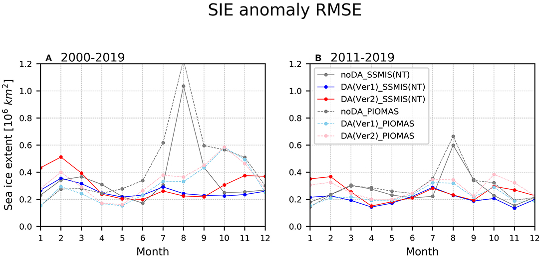
Figure 9. The root-mean-square-errors with respect to the SSMIS NT (solid lines) and PIOMAS (dashed lines) of sea ice extent index (106km2) for noDA (gray), Ver1 (blue and skyblue), and Ver2 (red and pink) during 2000–2019 (A) and 2011–2019 (B).
To investigate the time evolution of the SIE in more detail, we calculated the time-series of the SIE anomaly in February and August in Figure 10. In February, the noDA follows the overall variability well due to influence of the prescribed atmospheric and SST forcings (correlation coefficient between the SIE in noDA and SSMIS NT is 0.77) (Figure 10A). As noDA already exhibited a good performance, the positive impact of data assimilation on the interannual variability of SIE in February is minimal.
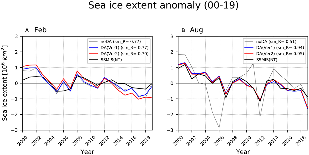
Figure 10. The time-series of Arctic sea ice extent anomaly (106km2) for SSMIS NT (black), noDA (gray), Ver1 (blue), and Ver2 (red) in February (A) and August (B) during 2000–2019. The “sm_R” in legend shows the correlation coefficient between each experiment and observation data.
However, in August, the quality of the reanalysis with the data assimilation is quite improved (Figure 10B). It is shown that the interannual variability of SIE in noDA is large in Figure 10B. We speculate that atmospheric forcing is the cause of large interannual variability in SIE in “noDA” in August. The downward shortwave radiation of the NCEP reanalysis data is relatively higher than that of other forcing data sets (e.g., JRA-55 and ERA-Interim) especially in summer, which may induce excessive melting of sea ice (Lee et al., 2019). As a result, it was understood that the thinning of sea ice due to the excessive shortwave radiation can lead to increased interannual variability of sea ice (Holland et al., 2008). The anomaly correlation coefficients between the noDA and the SSMIS NT is only 0.51, while the correlation with the SSMIS NT is improved to 0.94 (0.95) for Ver1 (Ver2).
In order to explore the regional features, we calculated the grid point-wise RMSE of the SIC anomalies during 2011–2019 in Figure 11. In February, the RMSEs of SIC in noDA, Ver1, and Ver2 against SSMIS NT tends to be similar from each other, which is consistent with the minimal improvement in simulating SIE in February. However, in August, the improvement by assimilating sea ice variables is clear. The RMSEs in noDA are systematically large over the overall Arctic regions, while that in Ver1 or Ver2 is significantly reduced in most regions (Figures 11D–F).
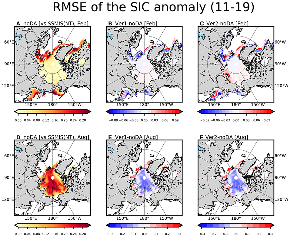
Figure 11. The root-mean-square-errors of sea ice concentration (a fraction from 0 to 1) for noDA, Ver1, and Ver2 with respect to the SSMIS NT observation are calculated in February (A–C) and in August (D–F). The RMSE of noDA (A,D) and the difference of Ver1 (B,E) and Ver2 (C,F) with respect to noDA are calculated during 2011–2019.
Figure 12 shows the RMSEs for the SIT anomalies in February and August in noDA, Ver1, and Ver2 against the CS2SMOS. In February, the noDA show that the RMSEs in CAP regions including east Greenland, Wandel Sea, and east of Beaufort Sea are relatively large than other regions (Figure 12A). In Ver1, the RMSE is slightly large over the polar regions compared to noDA (Figure 12B). In Ver2, the RMSE in CAP region is systematically reduced than that in noDA and Ver1 (Figure 12C). In August, the relatively large RMSEs are mainly shown over the CAP region in noDA, and it is relatively small in the remaining regions (Figure 12D). The RMSE of the SIT anomalies in Ver1 is increased to some extent compared to noDA (Figure 12E). Even though the RMSE of the SIT anomaly in Ver2 is systematically reduced than that in Ver1, however, it is only comparable to noDA (Figure 12F). This modest improvement is probably due to the fact that this is the season when the SIT observation is not injected even in Ver2 due to the lack of SIT observation.
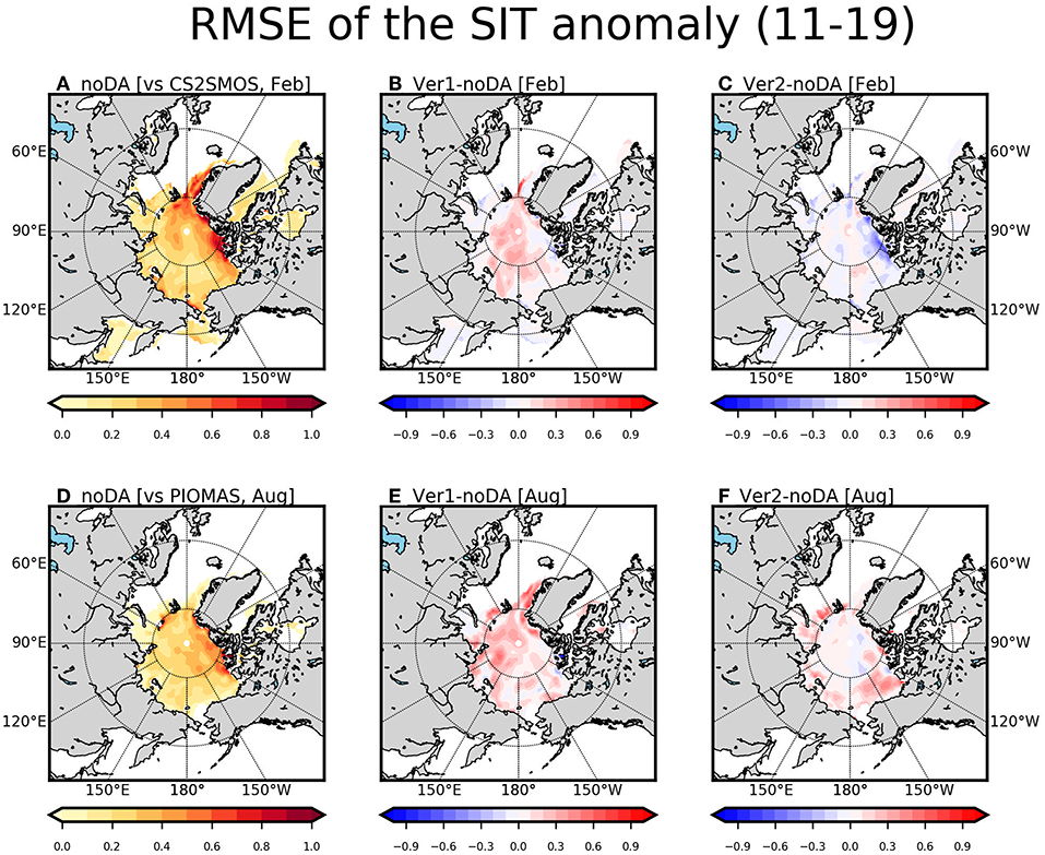
Figure 12. The root-mean-square-errors of sea ice thickness (m) for noDA, Ver1, and Ver2 with respect to the CS2SMOS observation and PIOMAS reanalysis are calculated in February (A–C) and in August (D–F). Note that the CS2SMOS is used in February and the PIOMAS is used in August due to the absence of satellite data. The RMSE of noDA (A,D) and the difference of Ver1 (B,E) and Ver2 (C,F) with respect to noDA are calculated during 2011–2019.
Dominant Modes
To analyze the spatial distribution of the dominant interannual variability of the SIC and SIT, we performed the empirical orthogonal function (EOF) analysis for observation and reanalysis. The leading EOF of SIC anomalies for SSMIS NT, PIOMAS, Ver1, and Ver2 in February for 2000–2019 are shown in Figure 13. The leading EOF for SSMIS NT, PIOMAS, Ver1, and Ver2 is well-separated from its second EOF and their explained variance is 23.2, 26.1, 24.4, and 32.5%, respectively. The leading EOF of SIC anomalies for SSMIS NT exhibits dipole patterns in the Greenland-Barents Sea and Baffin Bay-Labrador Seas in Atlantic sector (Figure 13A). The winter Odden sea ice feature, which denotes a large positive tongue of SIC anomaly that advances rapidly northeastward into the Greenland Sea over 8°W−5°E, 73–77°N (Shuchman et al., 1998; Deser et al., 2000), appears in all four products, even though those in the Ver1 and Ver2 exhibited a larger amplitude than the SSMIS NT or PIOMAS. The negative SIC anomalies are shown in Baffin Bay and Labrador Sea in all four products.
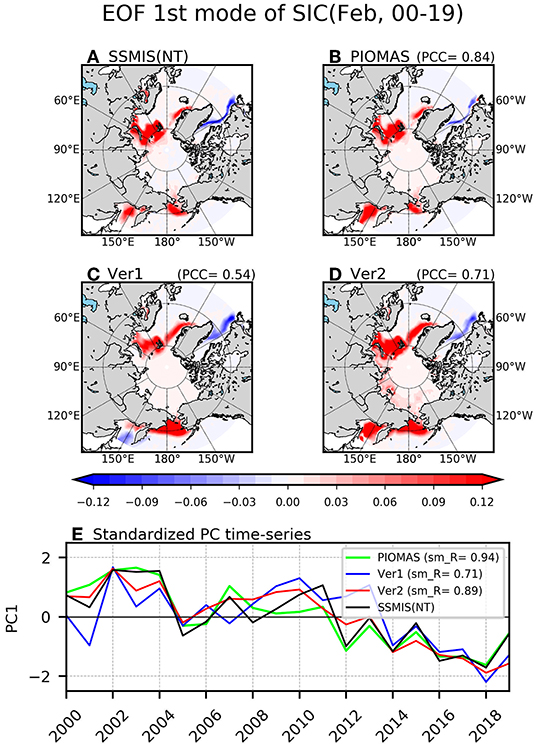
Figure 13. The spatial distributions of the eigenvector of the first empirical orthogonal function mode of sea ice concentration (a fraction from 0 to 1) for SSMIS NT observation (A), PIOMAS reanalysis (B), Ver1 (C), and Ver2 (D) in February during the period 2000–2019. The pattern correlation represented “PCC” is calculated between SSMIS NT observation and each product. The time-series of the principal component (E) for SSMIS NT (black), PIOMAS (light green), Ver1 (blue), and Ver2 (red) is calculated and the “sm_R” represents the correlation coefficients with SSMIS NT data.
In the Pacific sector, the positive SIC anomalies are shown over the Bering Sea in all four products. In the SSMIS NT and the PIOMAS, this SIC anomalies over the Bering Sea is mostly confined at the north of 60°N, whereas, in the Ver1 and Ver2, it is further extended to the south. The positive SIC anomalies appear in the Sea of Okhotsk in SSMIS NT, PIOMAS, and Ver2, however, it is overwhelmed by the negative values in Ver1. As a result, the SIC anomalies of the dominant EOF in Ver1 exhibited the erroneous dipole pattern. This is also shown in the dominant EOF in noDA (not shown), implying that the dipole pattern can be corrected through SIT data assimilation. In order to examine the similarity with the leading EOF of the SSMIS NT, we calculate the pattern correlation coefficients (PCC) for PIOMAS, Ver1 and Ver2. The dominant EOF in the PIOMAS is most similar to that in the SSMIS NT (PCC = 0.84), followed by Ver2 (0.71) and Ver1 (0.54).
The standardized principal component (PC) time series of the leading EOF for each data is shown in Figure 13E. All PC time series show a decreasing trend. The temporal correlation of the PC time-series from the SSMIS NT is almost similar between noDA and Ver1; the temporal correlation coefficient between the SSMIS NT and noDA is 0.86, where that between SSMIS NT and Ver1 is 0.72. However, assimilating SIT observation in Ver2 further improves the simulation quality of PC time-series (0.89). This means that the indirect effect of SIT data assimilation on SIC simulation contributes to the realistic SIC interannual variations.
The assimilation of the SIT observation plays a critical role in mimicking the observed leading EOF and the associated PC time series in February (Figure 14). The explained variance of the first modes accounts for 28.5, 28.5, 25.5, and 32.4%, for CS2SMOS, PIOMAS, Ver1, and Ver2, respectively. The CS2SMOS and PIOMAS shows that the interannual variability is robust over the CAP region (Figure 14A). In the CS2SMOS, a tongue of positive SIT anomaly extending from west to east in Beaufort Sea between 120°W and 180°E along the latitude of 71–74°N, associated with the Beaufort Gyre, is shown. However, the dominant EOF of the SIT in Ver1 exhibited quite different spatial distribution from the observation (Figure 14C). There is an arbitrary negative, and positive SIT anomalies near the CAP region, and Wandel Sea in Ver1, respectively. As a result, the PCC between the leading EOF in Ver1 and that of CS2SMOS is −0.27, and the correlation of the corresponding PC time-series is only 0.06 (Figure 14E). This clearly indicates the necessity of the SIT data assimilation for the realistic simulation of the SIT anomalies.
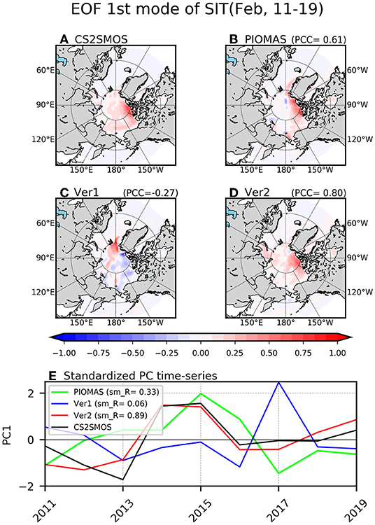
Figure 14. The first EOF mode of sea ice thickness in February during the period 2011−2019. The CS2SMOS satellite thickness data is used here. The arrangement of the plots is the same as in Figure 13.
On the other hand, in Ver2, the quality in simulating SIT anomalies is systematically improved (Figure 14D). The amplitude of the positive SIT anomalies in CAP region in Ver2 is similar to those in CS2SMOS. In addition, the zonally-elongated positive SIT anomalies associated with Beaufort Gyre is successfully mimicked to some extent only in Ver2. The PCC between the dominant EOF of CS2SMOS and that of Ver2 is 0.80, which exhibited even higher PCC value between CS2SMOS and PIOMAS (i.e., 0.61). The corresponding PC time-series in Ver2 is also well-correlated with the CS2SMOS (i.e., temporal correlation is 0.89) (Figure 14E). It appears that data assimilation of SIT significantly improves the simulation quality of dominant Arctic SIT variability during boreal winter.
The reanalysis quality in simulating SIC anomalies during boreal summer is quite similar between SSMIS NT, PIOMAS, Ver1, and Ver2 (not shown). On the other hand, the dominant EOF of the SIT anomalies in Ver2 exhibited a modest improvement during boreal summer (Figure 15). The leading EOF in PIOMAS shows the Central Arctic Thinning-like pattern (Fučkar et al., 2016) and the PCC between the dominant EOF of PIOMAS and that of Ver2 is 0.82, which exhibited slightly higher PCC between PIOMAS and Ver1 (i.e., 0.74). The corresponding PC time-series in Ver2 also exhibited higher temporal correlation with the PIOMAS (i.e., correlation is 0.87) than that in Ver1 (i.e., correlation is 0.72) (Figure 15D). As there is no observation of SIT in summer, the improvement in simulating SIT anomalies during boreal summer in Ver2 might be originated from the improved reanalysis quality of the SIT anomalies during boreal winter. That is, the realistic simulation of the SIT anomalies during boreal winter season is maintained up to boreal summer season possibly due to the multi-season persistency of the sea ice anomalies (Holland et al., 2011).
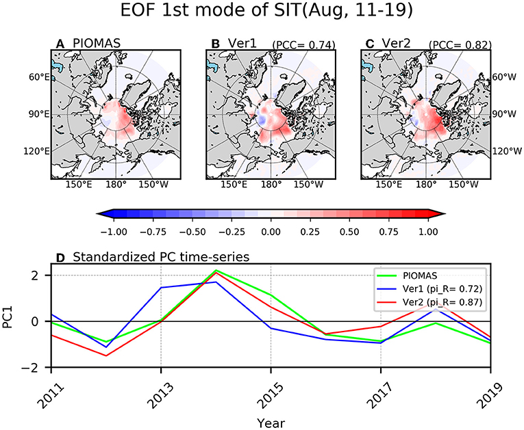
Figure 15. The spatial distribution of the eigenvector of first EOF mode of sea ice thickness for PIOMAS (A), Ver1 (B), and Ver2 (C) in August during 2011–2019. The pattern correlation represented “PCC” is calculated between PIOMAS and each experiment. The time-series of the principal component (D) for PIOMAS (light green), Ver1 (blue), and Ver2 (red) is calculated and the “pi_R” represents the correlation coefficients with PIOMAS reanalysis data.
Summary and Discussions
In this work, we have exploited the satellite observation of SIT from the CryoSat-2 and SMOS from European Space Agency’s (ESA), and SIC from the Special Sensor Microwave Imager/Sounder (SSMIS) aboard Defense Meteorological Satellite (DMSP) to assimilate the SIC and SIT in CICE5 model using ensemble optimal interpolation (EnOI). The SIC, and the SIT satellite observation are assimilated during 2000–2019, and 2011–2019, respectively. In order to use the EnOI, the stationary ensemble perturbations for calculating background error covariance matrix are generated by using long-term model integrations during 1982–2019. We have found that the stationary ensemble perturbations not only represent the seasonal variability of sea ice variable, but also successfully reflect the physical properties and balances related to the sea ice variability.
The quality of the reanalysis produced by sea ice data assimilation are evaluated in terms of climatological field, interannual variability, and dominant interannual variation by comparing assimilated states and the those in the observations and reanalysis. By assimilating the SIC satellite observations, the systematic bias of SIC in control simulation (i.e., noDA) is remarkably corrected in marginal ice zones, and pan-Arctic ocean during boreal winter, and summer season, respectively (Figure 6). The sea ice extent (SIE) anomalies in data assimilation experiments exhibited a similar year-to-year variation to SSMIS NT compared to that in noDA in all calendar months especially during boreal summer (Figures 9, 10). The SIC assimilation have an effect on the correction in climatological bias of SIT, but interannual variations of the SIT are still unrealistic (Figure 7), which requires an additional assimilation of SIT observation.
Not only the climatological bias, but also the RMSEs of SIT anomalies are further reduced particularly during boreal winter by additionally assimilating SIT observations (Figure 12). The empirical orthogonal function (EOF) analysis showed that the dominant interannual variation of SIT anomalies exhibited similar spatial distribution to those in the observation during boreal winter season (Figure 14). The positive SIT anomalies observed in central Arctic ocean, centered over the Canadian Archipelago (CAP), are well-simulated in Ver2 (experiment with SIC and SIT assimilation), where the negative anomalies are distributed in CAP and Beaufort Sea in Ver1 (experiment with SIC assimilation).
Interestingly, the improvement in the SIT states leads to the correction in the SIE bias (Figure 5). The reduction in the negative SIT bias by additionally assimilating SIT observation contributes to reduce the positive SIC bias over Kara-Barents Sea (Figure 8). This inverse relationship between SIC and SIT is also shown in the idealized experiment by increasing the SIT. Even though the assimilation of SIT observation did not result in appreciable differences in interannual variability of SIE anomalies, there has been the improvement in simulating dominant interannual variation for SIC in February (Figure 13). The observed dipole pattern between Greenland-Barents Sea and Baffin Bay-Labrador Sea, and the zonally-elongated positive SIC anomalies, referred as Odden feature, are well-simulated in reanalysis produced by both in Ver1 and Ver2. However, the observed positive anomalies in Sea of Okhotsk are successfully reproduced only in Ver2. The PC time-series of the leading EOF for SIC in Ver2 showed a higher temporal correlation with the observation than that in Ver1.
Through the series of the data assimilation of the sea ice variables, not only the degree of the improvement in simulating the climatology and the interannual variability of the sea ice can be assessed, but also a scientific question can be drawn. The indirect impact of the SIT assimilation on the SIC is one of typical subjects. The simulation of the SIC climatology and the variability tends to be improved once the SIT observation is further assimilated in addition to the SIC observation. This indicates that the non-linear physical processes associated with the corrected SIT help to improve the SIC simulation (Collow et al., 2015). In addition, even though the SIC improvement by assimilating SIT observation is not clear during boreal summer season in this study, several previous studies showed that the knowledge of winter ice thickness can provide some predictive capability for summer ice extent (Kauker et al., 2009; Holland et al., 2011). This means that the reduction the systematic errors in SIT during boreal winter season have a seasonal memory to improve the SIC simulation during boreal summer. To fully understand the mechanism of the improvement led by the data assimilation, the interactions between sea ice variables, and temporal memory of the sea ice variables, which might be dependent on the season, should be investigated further as a future work.
In addition, the improvement of the SIC simulation by assimilating SIT observation implies that the multi-variate assimilation might further improve the reanalysis quality. As it is already demonstrated that the updated SIT leads a positive impact on the SIC through physical processes in the model, the direct updates of the SIC by given SIT increment based on the modeled covariance would lead the improvement in simulating SIC without any time lags.
The reanalysis produced in this study aims to improve the quality of the initial condition of the sea ice component in the Global Seasonal forecast system (GloSea) for the seasonal forecasts (Maclachlan et al., 2015). In particular, as still operational version of the GloSea (i.e., GloSea version 5) for the seasonal forecasts only assimilates the SIC, the improvement in the sea ice initial conditions by assimilating the SIT observation is expected. This expectation is based on the previous studies that a significant improvement in predictive skill of Arctic sea-ice extent and ice edge location for multi-seasons forecasts targeted to September Arctic sea ice by assimilating the CryoSat-2 thickness (Blockley and Andrew Peterson, 2018). However, the temporal coverage of the SIT observation is limited after 2010, and this significantly shortens the hindcasts period compared to the conventional period for the hindcasts for seasonal forecasts (i.e., longer than two decades, e.g., Johnson et al., 2019). Nonetheless, the temporal coverage of a decade (i.e., from 2010 to the present) would allow the preliminary assessment of the seasonal forecast skill and its possible advantages by assimilating the SIT observations.
Data Availability Statement
The original contributions presented in the study are included in the article, further inquiries can be directed to the corresponding author.
Author Contributions
J-GL and Y-GH designed the research and wrote the paper. J-GL performed the experiments and analyzed the data. Both authors discussed the methodology, results and structure of the paper. Both authors contributed to the article and approved the submitted version.
Funding
This study was supported by the Korea Meteorological Administration Research and Development Program under Grant KMI2021-01210.
Conflict of Interest
The authors declare that the research was conducted in the absence of any commercial or financial relationships that could be construed as a potential conflict of interest.
Publisher’s Note
All claims expressed in this article are solely those of the authors and do not necessarily represent those of their affiliated organizations, or those of the publisher, the editors and the reviewers. Any product that may be evaluated in this article, or claim that may be made by its manufacturer, is not guaranteed or endorsed by the publisher.
Acknowledgments
We thank the NSIDC for providing SSMIS sea ice concentration (http://nsidc.org/data/nsidc-0051 and nsidc-0079), CryoSat-2 sea ice thickness (http://nsidc.org/data/RDEFT4), the University of Hamburg for providing SMOS sea ice thickness (https://icdc.cen.uni-hamburg.de/thredds/catalog/ftpthredds/smos_sea_ice_thickness/catalog.html), and the Alfred Wegener Institute for sharing CS2SMOS sea ice thickness (https://spaces.awi.de/display/CS2SMOS/). NCEP_Reanalysis 2 and OISST V2 data were provided by the National Oceanic and Atmospheric Administration (NOAA) and the PIOMAS reanalysis is provided by Polar Science Center.
References
Aksenov, Y., Popova, E. E., Yool, A., Nurser, A. J. G., Williams, T. D., Bertino, L., et al. (2017). On the future navigability of Arctic sea routes: high-resolution projections of the Arctic Ocean and sea ice. Mar. Policy 75, 300–317. doi: 10.1016/j.marpol.2015.12.027
Backeberg, B. C., Counillon, F., Johannessen, J. A., and Pujol, M. I. (2014). Assimilating along-track sla data using the EnOI in an eddy resolving model of the agulhas system. Ocean Dyn. 64, 1121–1136. doi: 10.1007/s10236-014-0717-6
Bader, J., Mesquita, M. D. S., Hodges, K. I., Keenlyside, N., Østerhus, S., and Miles, M. (2011). A review on Northern Hemisphere sea-ice, storminess and the North Atlantic Oscillation: observations and projected changes. Atmos. Res. 101, 809–834. doi: 10.1016/j.atmosres.2011.04.007
Blackport, R., and Screen, J. A. (2020a). Insignificant effect of Arctic amplification on the amplitude of midlatitude atmospheric waves. Sci. Adv. 6, 1–10. doi: 10.1126/sciadv.aay2880
Blanchard-Wrigglesworth, E., Cullather, R. I., Wang, W., Zhang, J., and Bitz, C. M. (2015). Model forecast skill and sensitivity to initial conditions in the seasonal Sea Ice Outlook. Geophys. Res. Lett. 42, 8042–8048. doi: 10.1002/2015GL065860
Blockley, E. W., and Andrew Peterson, K. (2018). Improving Met Office seasonal predictions of Arctic sea ice using assimilation of CryoSat-2 thickness. Cryosphere 12, 3419–3438. doi: 10.5194/tc-12-3419-2018
Cavalieri, D. J., Parkinson, C. L., Gloersen, P., and Zwally, H. J. (1996). Sea Ice Concentrations From Nimbus-7 SMMR and DMSP SSM/I-SSMIS Passive Microwave Data, Version 1. [NSIDC-0051]. Boulder, CO: National Snow and Ice Data Center, 0–29. Available online at: https://nsidc.org/data/NSIDC-0051/ (accessed February 2, 2022).
Caya, A., Buehner, M., and Carrieres, T. (2010). Analysis and forecasting of sea ice conditions with three-dimensional variational data assimilation and a coupled ice-ocean model. J. Atmos. Ocean. Technol. 27, 353–369. doi: 10.1175/2009JTECHO701.1
Chen, Z., Liu, J., Song, M., Yang, Q., and Xu, S. (2017). Impacts of assimilating satellite sea ice concentration and thickness on Arctic sea ice prediction in the NCEP climate forecast system. J. Clim. 30, 8429–8446. doi: 10.1175/JCLI-D-17-0093.1
Chevallier, M., Mélia, D. S. Y., Voldoire, A., Déqué, M., and Garric, G. (2013). Seasonal forecasts of the pan-arctic sea ice extent using a GCM-based seasonal prediction system. J. Clim. 26, 6092–6104. doi: 10.1175/JCLI-D-12-00612.1
Cohen, J., Zhang, X., Francis, J., Jung, T., Kwok, R., Overland, J., et al. (2020). Divergent consensuses on Arctic amplification influence on midlatitude severe winter weather. Nat. Clim. Change 10, 20–29. doi: 10.1038/s41558-019-0662-y
Cohen, J. L., Furtado, J. C., Barlow, M. A., Alexeev, V. A., and Cherry, J. E. (2012). Arctic warming, increasing snow cover and widespread boreal winter cooling. Environ. Res. Lett. 7, 14007. doi: 10.1088/1748-9326/7/1/014007
Collow, T. W., Wang, W., Kumar, A., and Zhang, J. (2015). Improving arctic sea ice prediction using PIOMAS initial sea ice thickness in a coupled ocean-atmosphere model. Mon. Weather Rev. 143, 4618–4630. doi: 10.1175/MWR-D-15-0097.1
Comiso, J. C. (2017). Bootstrap Sea Ice Concentrations From Nimbus-7 SMMR and DMSP SSM/I-SSMIS, Version 3 [NSIDC-0079]. Boulder, CO: National Snow and Ice Data Center, 14. Available online at: https://nsidc.org/data/nsidc-0079/ (accessed February 2, 2022).
Danabasoglu, G., Lamarque, J. F., Bacmeister, J., Bailey, D. A., DuVivier, A. K., Edwards, J., et al. (2020). The community earth system model version 2 (CESM2). J. Adv. Model. Earth Syst. 12, 1–35. doi: 10.1029/2019MS001916
Deser, C., Tomas, R. A., and Sun, L. (2015). The role of ocean-atmosphere coupling in the zonal-mean atmospheric response to Arctic sea ice loss. J. Clim. 28, 2168–2186. doi: 10.1175/JCLI-D-14-00325.1
Deser, C., Walsh, J. E., and Timlin, M. S. (2000). Arctic sea ice variability in the context of recent atmospheric circulation trends. J. Clim. 13, 617–633. doi: 10.1175/1520-0442(2000)013<0617:ASIVIT>2.0.CO;2
Ding, Q., Schweiger, A., L’Heureux, M., Battisti, D. S., Po-Chedley, S., Johnson, N. C., et al. (2017). Influence of high-latitude atmospheric circulation changes on summertime Arctic sea ice. Nat. Clim. Change 7, 289–295. doi: 10.1038/nclimate3241
Dirkson, A., Merryfield, W. J., and Monahan, A. H. (2019). Calibrated probabilistic forecasts of Arctic sea ice concentration. J. Clim. 32, 1251–1271. doi: 10.1175/JCLI-D-18-0224.1
Evensen, G. (2003). The ensemble kalman filter: theoretical formulation and practical implementation. Ocean Dyn. 53, 343–367. doi: 10.1007/s10236-003-0036-9
Fritzner, S., Graversen, R., Christensen, K., Rostosky, P., and Wang, K. (2019). Impact of assimilating sea ice concentration, sea ice thickness and snow depth in a coupled ocean-sea ice modelling system. Cryosphere 13, 491–509. doi: 10.5194/tc-13-491-2019
Fučkar, N. S., Guemas, V., Johnson, N. C., Massonnet, F., and Doblas-Reyes, F. J. (2016). Clusters of interannual sea ice variability in the northern hemisphere. Clim. Dyn. 47, 1527–1543. doi: 10.1007/s00382-015-2917-2
Gao, P. A., Director, H. M., Bitz, C. M., and Raftery, A. E. (2021). Probabilistic forecasts of Arctic sea ice thickness. J. Agric. Biol. Environ. Stat. 1–23. doi: 10.1007/s13253-021-00480-0
Gaspari, G., and Cohn, S. E. (1999). Construction of correlation functions in two and three dimensions. Q. J. R. Meteorol. Soc. 125, 723–757. doi: 10.1002/qj.49712555417
Gent, P. R., Danabasoglu, G., Donner, L. J., Holland, M. M., Hunke, E. C., Jayne, S. R., et al. (2011). The community climate system model version 4. J. Clim. 24, 4973–4991. doi: 10.1175/2011JCLI4083.1
Goosse, H., Arzel, O., Bitz, C. M., De Montety, A., and Vancoppenolle, M. (2009). Increased variability of the Arctic summer ice extent in a warmer climate. Geophys. Res. Lett. 36, 1–5. doi: 10.1029/2009GL040546
Guarino, M. V., Sime, L. C., Schröeder, D., Malmierca-Vallet, I., Rosenblum, E., Ringer, M., et al. (2020). Sea-ice-free Arctic during the Last Interglacial supports fast future loss. Nat. Clim. Chang. 10, 928–932. doi: 10.1038/s41558-020-0865-2
Hendricks, S., Paul, S., and Rinne, E. (2018). ESA Sea Ice Climate Change Initiative (Sea_Ice_cci): Northern Hemisphere Sea Ice Thickness From Envisat on the Satellite Swath (L2P), v2.0. Centre for Environmental Data Analysis. doi: 10.5285/54e2ee0803764b4e84c906da3f16d81b
Holland, M. M., Bailey, D. A., and Vavrus, S. (2011). Inherent sea ice predictability in the rapidly changing Arctic environment of the Community Climate System Model, version 3. Clim. Dyn. 36, 1239–1253. doi: 10.1007/s00382-010-0792-4
Holland, M. M., Bitz, C. M., Tremblay, L. B., and Bailey, D. A. (2008). The role of natural versus forced change in future rapid summer arctic ice loss. Geophys. Monogr. Ser. 180, 133–150. doi: 10.1029/180GM10
Hunke, E. C., Lipscomb, W. H., Turner, A. K., Jeffery, N., and Elliott, S. (2015). CICE: The Los Alamos Sea Ice Model Documentation and Software User’s Manual Version 5.1. LA-CC-06–012. Los Alamos, NM: Los Alamos National Laboratory. Available online at: http://www.ccpo.odu.edu/~klinck/Reprints/PDF/cicedoc2015.pdf (accessed March 17, 2015).
Hunt, B. R., Kostelich, E. J., and Szunyogh, I. (2007). Efficient data assimilation for spatiotemporal chaos: A local ensemble transform Kalman filter. Phys. D Nonlinear Phenom. 230, 112–126. doi: 10.1016/j.physd.2006.11.008
Hurrell, J. W., Holland, M. M., Gent, P. R., Ghan, S., Kay, J. E., Kushner, P. J., et al. (2013). The community earth system model: A framework for collaborative research. Bull. Am. Meteorol. Soc. 94, 1339–1360. doi: 10.1175/BAMS-D-12-00121.1
Janjić, T., Bormann, N., Bocquet, M., Carton, J. A., Cohn, S. E., Dance, S. L., et al. (2018). On the representation error in data assimilation. Q. J. R. Meteorol. Soc. 144, 1257–1278. doi: 10.1002/qj.3130
Johnson, S. J., Stockdale, T. N., Ferranti, L., Balmaseda, M. A., Molteni, F., Magnusson, L., et al. (2019). SEAS5: the new ECMWF seasonal forecast system. Geosci. Model Dev. 12, 1087–1117. doi: 10.5194/gmd-12-1087-2019
Kaleschke, L., Tian-Kunze, X., Maaß, N., Beitsch, A., Wernecke, A., Miernecki, M., et al. (2016). SMOS sea ice product: operational application and validation in the Barents Sea marginal ice zone. Remote Sens. Environ. 180, 264–273. doi: 10.1016/j.rse.2016.03.009
Kaleschke, L., Tian-Kunze, X., Maaß, N., Mäkynen, M., and Drusch, M. (2012). Sea ice thickness retrieval from SMOS brightness temperatures during the Arctic freeze-up period. Geophys. Res. Lett. 39, 1–5. doi: 10.1029/2012GL050916
Kanamitsu, M., Ebisuzaki, W., Woollen, J., Yang, S., Hnilo, J. J., Fiorino, M., et al. (2002). NCEP–DOE AMIP-II Reanalysis (R-2). Bull. Am. Meteorol. Soc. 83, 1631–1644. doi: 10.1175/BAMS-83-11-1631
Kauker, F., Kaminski, T., Karcher, M., Giering, R., Gerdes, R., and Voßbeck, M. (2009). Adjoint analysis of the 2007 all time Arctic sea-ice minimum. Geophys. Res. Lett. 36, 1–5. doi: 10.1029/2008GL036323
Kaurkin, M. N., Ibrayev, R. A., and Belyaev, K. P. (2016). ARGO data assimilation into the ocean dynamics model with high spatial resolution using Ensemble Optimal Interpolation (EnOI). Oceanology 56, 774–781. doi: 10.1134/S0001437016060059
Kim, B. M., Son, S. W., Min, S. K., Jeong, J. H., Kim, S. J., Zhang, X., et al. (2014). Weakening of the stratospheric polar vortex by Arctic sea-ice loss. Nat. Commun. 5, 5646. doi: 10.1038/ncomms5646
Kimmritz, M., Counillon, F., Bitz, C. M., Massonnet, F., Bethke, I., and Gao, Y. (2018). Optimising assimilation of sea ice concentration in an Earth system model with a multicategory sea ice model. Tellus, Ser. A Dyn. Meteorol. Oceanogr. 70, 1–23. doi: 10.1080/16000870.2018.1435945
Kinnard, C., Zdanowicz, C. M., Fisher, D. A., Isaksson, E., de Vernal, A., and Thompson, L. G. (2011). Reconstructed changes in Arctic sea ice over the past 1,450 years. Nature 479, 509–512. doi: 10.1038/nature10581
Kug, J. S., Jeong, J. H., Jang, Y. S., Kim, B. M., Folland, C. K., Min, S. K., et al. (2015). Two distinct influences of Arctic warming on cold winters over North America and East Asia. Nat. Geosci. 8, 759–762. doi: 10.1038/ngeo2517
Kurtz, N., and Harbeck, J. (2017). CryoSat-2 Level-4 Sea Ice Elevation, Freeboard, and Thickness, Version 1. Boulder, CO: NASA Natl. Snow Ice Data Cent. Distrib. Act. Arch. Center, 0–9. Available online at: https://nsidc.org/data/RDEFT4/ (accessed February 2, 2022).
Kurtz, N. T., Galin, N., and Studinger, M. (2014). An improved CryoSat-2 sea ice freeboard retrieval algorithm through the use of waveform fitting. Cryosphere 8, 1217–1237. doi: 10.5194/tc-8-1217-2014
Kwok, R. (2018). Arctic sea ice thickness, volume, and multiyear ice coverage: Losses and coupled variability (1958-2018). Environmental Research Letters 13. doi: 10.1088/1748-9326/aae3ec
Kwok, R., and Rothrock, D. A. (2009). Decline in Arctic sea ice thickness from submarine and ICESat records: 1958-2008. Geophys. Res. Lett. 36, 1–5. doi: 10.1029/2009GL039035
Large, W. G., and Yeager, S. G. (2009). The global climatology of an interannually varying air – Sea flux data set. Clim. Dyn. 33, 341–364. doi: 10.1007/s00382-008-0441-3
Lee, S. B., Kim, B. M., Ukita, J., and Ahn, J. B. (2019). Uncertainties in arctic sea ice thickness associated with different atmospheric reanalysis datasets using the CICE5 model. Atmosphere 10, 1–15. doi: 10.3390/atmos10070361
Lindsay, R. W., and Zhang, J. (2006). Assimilation of ice concentration in an ice-ocean model. J. Atmos. Ocean. Technol. 23, 742–749. doi: 10.1175/JTECH1871.1
Lisæter, K. L., Rosanova, J., and Evensen, G. (2003). Assimilation of ice concentration in a coupled ice-ocean model, using the Ensemble Kalman filter. Ocean Dyn. 53, 368–388. doi: 10.1007/s10236-003-0049-4
Liu, M., and Kronbak, J. (2010). The potential economic viability of using the Northern Sea Route (NSR) as an alternative route between Asia and Europe. J. Transp. Geogr. 18, 434–444. doi: 10.1016/j.jtrangeo.2009.08.004
Maclachlan, C., Arribas, A., Peterson, K. A., Maidens, A., Fereday, D., Scaife, A. A., et al. (2015). Global Seasonal forecast system version 5 (GloSea5): a high-resolution seasonal forecast system. Q. J. R. Meteorol. Soc. 141, 1072–1084. doi: 10.1002/qj.2396
Martin, T. (2007). Arctic sea ice dynamics: drift and ridging in numerical models and observations (dissertation), University of Bremen, Bremen.
Massonnet, F., Fichefet, T., and Goosse, H. (2015). Prospects for improved seasonal Arctic sea ice predictions from multivariate data assimilation. Ocean Model 88, 16–25. doi: 10.1016/j.ocemod.2014.12.013
Massonnet, F., Mathiot, P., Fichefet, T., Goosse, H., König Beatty, C., Vancoppenolle, M., et al. (2013). A model reconstruction of the Antarctic sea ice thickness and volume changes over 1980-2008 using data assimilation. Ocean Model. 64, 67–75. doi: 10.1016/j.ocemod.2013.01.003
Massonnet, F., Vancoppenolle, M., Goosse, H., Docquier, D., Fichefet, T., and Blanchard-Wrigglesworth, E. (2018). Arctic sea-ice change tied to its mean state through thermodynamic processes. Nat. Clim. Change 8, 599–603. doi: 10.1038/s41558-018-0204-z
Mignac, D., Tanajura, C. A. S., Santana, A. N., Lima, L. N., and Xie, J. (2015). Argo data assimilation into HYCOM with an EnOI method in the Atlantic Ocean. Ocean Sci. 11, 195–213. doi: 10.5194/os-11-195-2015
Mori, M., Watanabe, M., Shiogama, H., Inoue, J., and Kimoto, M. (2014). Robust Arctic sea-ice influence on the frequent Eurasian cold winters in past decades. Nat. Geosci. 7, 869–873. doi: 10.1038/ngeo2277
Mu, L., Yang, Q., Losch, M., Losa, S. N., Ricker, R., Nerger, L., et al. (2018). Improving sea ice thickness estimates by assimilating CryoSat-2 and SMOS sea ice thickness data simultaneously. Q. J. R. Meteorol. Soc. 144, 529–538. doi: 10.1002/qj.3225
Notz, D., Dörr, J., Bailey, D. A., Blockley, E., Bushuk, M., Debernard, J. B., et al. (2020). Arctic Sea Ice in CMIP6. Geophys. Res. Lett. 47, e2019GL086749. doi: 10.1029/2019GL086749
Oke, P. R., Sakov, P., and Corney, S. P. (2007). Impacts of localisation in the EnKF and EnOI: experiments with a small model. Ocean Dyn. 57, 32–45. doi: 10.1007/s10236-006-0088-8
Overland, J. E., Adams, J. M., and Bond, N. A. (1999). Decadal variability of the Aleutian low and its relation to high-latitude circulation. J. Clim. 12, 1542–1548. doi: 10.1175/1520-0442(1999)012<1542:DVOTAL>2.0.CO;2
Overland, J. E., Dethloff, K., Francis, J. A., Hall, R. J., Hanna, E., Kim, S. J., et al. (2016). Nonlinear response of mid-latitude weather to the changing Arctic. Nat. Clim. Change 6, 992–999. doi: 10.1038/nclimate3121
Perovich, D., Meier, W., Tschudi, M., Farrell, S., Hendricks, S., Gerland, C. H., et al. (2017). Sea Ice [in Arctic Report Card]. Available online at: https://www.arctic.noaa.gov/Report-Card/Report-Card-2017 (accessed February 2, 2022).
Rayner, N. A., Parker, D. E., Horton, E. B., Folland, C. K., Alexander, L. V., et al. (2003). Global analyses of sea surface temperature, sea ice, and night marine air temperature since the late nineteenth century. J. Geophys. Res. 108:2670. doi: 10.1029/2002JD002670
Reynolds, R. W., Rayner, N. A., Smith, T. M., Stokes, D. C., and Wang, W. (2002). An improved in situ and satellite SST analysis for climate. J. Clim. 15, 1609–1625. doi: 10.1175/1520-0442(2002)015<1609:AIISAS>2.0.CO;2
Ricker, R., Hendricks, S., Kaleschke, L., Tian-Kunze, X., King, J., and Haas, C. (2017). A weekly Arctic Sea-ice thickness data record from merged CryoSat-2 and SMOS satellite data. Cryosph. Discuss. 11, 1607–1623. doi: 10.5194/tc-11-1607-2017
Sakov, P., and Bertino, L. (2011). Relation between two common localisation methods for the EnKF. Comput. Geosci. 15, 225–237. doi: 10.1007/s10596-010-9202-6
Semenov, V. A., Martin, T., Behrens, L. K., and Latif, M. (2015). Arctic sea ice area in CMIP3 and CMIP5 climate model ensembles – variability and change. Cryosphere 9, 1077–1131. doi: 10.5194/tcd-9-1077-2015
Serreze, M. C., Barrett, A. P., Stroeve, J. C., Kindig, D. N., and Holland, M. M. (2009). The emergence of surface-based Arctic amplification. Cryosphere 3, 11–19. doi: 10.5194/tc-3-11-2009
Shuchman, A., Josberger, G., Russel, A., Fischer, W., and Johannessen, M. (1998). The Greenland Sea odden sea ice feature: intra- and inter-annual variability. J. Geophys. Res. 103, 12709–12724. doi: 10.1029/98JC00375
Sigmond, M., Fyfe, J. C., Flato, G. M., Kharin, V. V., and Merryfield, W. J. (2013). Seasonal forecast skill of Arctic sea ice area in a dynamical forecast system. Geophys. Res. Lett. 40, 529–534. doi: 10.1002/grl.50129
Smith, L. C., and Stephenson, S. R. (2013). New Trans-Arctic shipping routes navigable by midcentury. Proc. Natl. Acad. Sci. U.S.A. 110, 6–10. doi: 10.1073/pnas.1214212110
Stark, J. D., Ridley, J., Martin, M., and Hines, A. (2008). Sea ice concentration and motion assimilation in a sea ice-ocean model. J. Geophys. Res. Ocean. 113, 1–19. doi: 10.1029/2007JC004224
Stroeve, J. C., Kattsov, V., Barrett, A., Serreze, M., Pavlova, T., Holland, M., et al. (2012a). Trends in Arctic sea ice extent from CMIP5, CMIP3 and observations. Geophys. Res. Lett. 39, 1–7. doi: 10.1029/2012GL052676
Stroeve, J. C., Serreze, M. C., Holland, M. M., Kay, J. E., Malanik, J., and Barrett, A. P. (2012b). The Arctic’s rapidly shrinking sea ice cover: a research synthesis. Clim. Change 110, 1005–1027. doi: 10.1007/s10584-011-0101-1
Tian-Kunze, X., Kaleschke, L., Maaß, N., Mäkynen, M., Serra, N., Drusch, M., et al. (2014). SMOS-derived thin sea ice thickness: algorithm baseline, product specifications and initial verification. Cryosphere 8, 997–1018. doi: 10.5194/tc-8-997-2014
Tietsche, S., Day, J. J., Guemas, V., Hurlin, W. J., Keeley, S. P. E., Matei, D., et al. (2014). Seasonal to interannual Arctic sea ice predictability in current global climate models. Geophys. Res. Lett. 41, 1035–1043. doi: 10.1002/2013GL058755
Tietsche, S., Notz, D., Jungclaus, J. H., and Marotzke, J. (2013). Assimilation of sea-ice concentration in a global climate model-physical and statistical aspects. Ocean Sci. 9, 19–36. doi: 10.5194/os-9-19-2013
Tilling, R. L., Ridout, A., and Shepherd, A. (2018). Estimating Arctic sea ice thickness and volume using CryoSat-2 radar altimeter data. Adv. Space Res. 62, 1203–1225. doi: 10.1016/j.asr.2017.10.051
Tonboe, R., and Nielsen, E. (2010). Ocean & Sea Ice SAF Global Sea Ice Concentration Reprocessing Validation Report. Copenhagen: Rasmus Tonboe and Esben Nielsen Danish Meteorological Institute. 1–17.
Toth, Z., and Kalnay, E. (1993). Ensemble forecasting at NMC: the generation of perturbations. Bull. Am. Meteorol. Soc. 74, 2317–2330. doi: 10.1175/1520-0477(1993)074<2317:EFANTG>2.0.CO;2
Toth, Z., and Kalnay, E. (1997). Ensemble forecasting at NCEP and the breeding method. Mon. Weather Rev. 125, 3297–3319. doi: 10.1175/1520-0493(1997)125<3297:EFANAT>2.0.CO;2
Turner, A. K., Hunke, E. C., and Bitz, C. M. (2013). Two modes of sea-ice gravity drainage: A parameterization for large-scale modeling. J. Geophys. Res. Ocean. 118, 2279–2294. doi: 10.1002/jgrc.20171
Wang, M., and Overland, J. E. (2012). A sea ice free summer Arctic within 30 years: An update from CMIP5 models. Geophys. Res. Lett. 39, 6–11. doi: 10.1029/2012GL052868
Wang, W., Chen, M., and Kumar, A. (2013). Seasonal prediction of arctic sea ice extent from a coupled dynamical forecast system. Mon. Weather Rev. 141, 1375–1394. doi: 10.1175/MWR-D-12-00057.1
Wayand, N. E., Bitz, C. M., and Blanchard-Wrigglesworth, E. (2019). A year-round subseasonal-to-seasonal sea ice prediction portal. Geophys. Res. Lett. 46, 3298–3307. doi: 10.1029/2018GL081565
Wilchinsky, A. V., and Feltham, D. L. (2006). Modelling the rheology of sea ice as a collection of diamond-shaped floes. J. Nonnewton. Fluid Mech. 138, 22–32. doi: 10.1016/j.jnnfm.2006.05.001
Xie, J., Counillon, F., and Bertino, L. (2018). Impact of assimilating a merged sea-ice thickness from CryoSat-2 and SMOS in the Arctic reanalysis. Cryosphere 12, 3671–3691. doi: 10.5194/tc-12-3671-2018
Yang, Q., Losa, S. N., Losch, M., Tian-Kunze, X., Nerger, L., Liu, J., et al. (2014). Assimilating SMOS sea ice thickness into a coupled ice-ocean model using a local SEIK filter. J. Geophys. Res. Ocean. 119, 6680–6692. doi: 10.1002/2014JC009963
Zhang, J., and Rothrock, D. A. (2003). Modeling global sea ice with a thickness and enthalpy distribution model in generalized curvilinear coordinates. Mon. Weather Rev. 131, 845–861. doi: 10.1175/1520-0493(2003)131<0845:MGSIWA>2.0.CO;2
Zhang, X., Lu, C., and Guan, Z. (2012). Weakened cyclones, intensified anticyclones and recent extreme cold winter weather events in Eurasia. Environ. Res. Lett. 7, 044044. doi: 10.1088/1748-9326/7/4/044044
Zhang, Y. F., Bitz, C. M., Anderson, J. L., Collins, N., Hendricks, J., Hoar, T., et al. (2018). Insights on Sea Ice data assimilation from perfect model observing system simulation experiments. J. Clim. 31, 5911–5926. doi: 10.1175/JCLI-D-17-0904.1
[ad_2]