A Double-Layer Optimization Maintenance Strategy for Photovoltaic Power Generation Systems Considering Component Correlation and Availability
[ad_1]
Introduction
The operating environment of photovoltaic power plants is complex, and the availability of each component is easily affected by various random and uncertain factors. Therefore, formulating reasonable and effective maintenance strategies is of great significance to the safe, economical, and stable operation of photovoltaic power plants.
The maintenance strategy of photovoltaic power generation systems is mainly divided into post-maintenance and preventive maintenance. Post-maintenance will cause varying degrees of damage to components and systems, thereby reducing their reliability. Preventive maintenance has over-repair and under-repair problems and cannot take into account the requirements of repair costs and optimal availability. At present, research on maintenance strategies of photovoltaic power generation systems mainly focuses on optimizing the maintenance time intervals, maintenance based on condition monitoring and prediction, and failure correlation analysis. In the work by Spertino et al. (2021), the effects of maintenance activities, reliability, and availability of photovoltaic systems on energy loss are described, but specific maintenance strategies are not given. Perdue and Gottschalg (2015) analyzed the relationship between the maintenance cycle and maintenance cost and concluded that the longer the maintenance cycle, the lower the maintenance cost, and the lower the reliability. In the work by Gunda et al. (2020), the failure types of equipment are distinguished by machine learning, which lays the foundation for formulating condition-based maintenance strategies. In the work by Mengying et al. (2021), a phased approach for periodic inspection and maintenance is proposed, and preventive maintenance is performed on equipment that is at risk of failure after inspection. In the work by Colombi Gomes and Rodrigues Muniz (2020), an economically optimized maintenance scheme is proposed, but this method is a preventively planned maintenance for cleaning the main dust of PV modules and fails to take into account the whole PV plant. Mahani et al. (2018) proposed a maintenance method of double-layer optimization of the microgrid, which has a certain contribution in reducing the waste of funds but fails to take into account the influence of reliability and so on. In the work by Sun and Sun (2021), a selective maintenance scheme considering the maintenance sequence is proposed; the model improves the reliability of the system to a certain extent, but the maintenance effect weakens with the extension of the maintenance cycle. The aforementioned research mainly determined the maintenance time or cycle with the goal of optimizing the maintenance cost. However, it failed to consider the influence of the operating state of the equipment and the related characteristics between the equipment on the maintenance strategy. If the influence is ignored, the error of maintenance time will be caused, which will increase the extra maintenance cost and reduce the availability of the system. Therefore, some scholars formulate maintenance strategies by considering the operational status of the equipment and the economic and structural dependencies of components. Verbert et al. (2017) determined the maintenance time and period through condition prediction based on the economic relevance of components. In the work by Li et al. (2021), taking reliability as a constraint, preventive opportunistic maintenance is performed on components by updating maintenance thresholds. In the work by Zhao et al. (2016), a state-opportunistic maintenance strategy is proposed by considering incomplete maintenance, which is widely used in the maintenance field as a typical form of preventive maintenance. Zhu and Liu (2020) proposed a maintenance strategy based on the hierarchical optimization of components and systems; the optimal maintenance strategy is derived by determining the maintenance time of components and systems. In the work by Xu et al. (2015), a condition-based maintenance model is proposed considering the functional correlation between components. In the work by Liu et al. (2015), the process of equipment deterioration and fault evolution is described by the Markov state transition equation, and the maintenance method and time interval are determined by the minimum maintenance cost. In the work by Catelani et al. (2020), a data-driven condition monitoring method and reliability-centered maintenance are proposed, but this method mainly emphasizes reliability analysis and fails to clearly point out the maintenance strategy. Oprea et al. (2019) calculated the reliability index by designing a probabilistic model based on Markov chain and proposed maintenance activities based on this to optimize the inventory of spare parts. Xu et al. (2017) predicted the future degradation and change process of the equipment based on the operation data of the equipment; an optimized maintenance program with the goal of optimizing profit is established. In the work by Wang et al. (2018), an incomplete maintenance model is proposed by considering the process of equipment degradation and shock but fails to consider the impact of special environments on maintenance strategies.
The aforementioned literatures took into account the economic and structural dependencies and state transition processes of equipment. Preventive maintenance was carried out through state prediction. Compared with regular maintenance, the aforementioned research improved the operation and maintenance efficiency and reduced the maintenance cost but failed to consider the impact of failure correlation. In terms of failure correlation, scholars mainly study the mutual influence of failure rates (Peng et al., 2020; Nguyen et al., 2019). When the relationship of fault influence is not clear, the Copula function is usually used to describe the correlation (Xu et al., 2020; Zhu et al., 2019). In the work by Fu et al. (2019), the failure correlation between components was analyzed by the Copula function, and a joint risk model based on failure interaction was established. In the work by Song et al. (2014), a reliability model was established by considering the fault correlation between components. The aforementioned research studies are mainly in the field of mechanical engineering and other fields of fault correlation analysis. However, in the field of photovoltaic operation and maintenance, the research on maintenance strategies considering fault correlation is still in its infancy.
The formulation of the maintenance strategy in existing research studies is mainly based on the operating state of the equipment, and the reliability is used as a constraint to judge whether maintenance is required, and then the maintenance strategy is optimized on the basis of considering maintenance costs. These maintenance methods reduce maintenance costs to a certain extent. However, it fails to take into account the impact of availability and comprehensive correlation and does not take into account the impact of weather factors on maintenance costs and system availability. Therefore, the maintenance plan formulated is not necessarily the best maintenance plan for the system. Thus, the maximum efficiency of photovoltaic power generation cannot be guaranteed. In view of the aforementioned problems, this study first analyzes the functional dependencies and failure transfer process of equipment in photovoltaic power plants. Then, it combines the Copula theory and Sklar theorem to describe the failure correlation characteristics between devices and models the availability of the system and components by improving the Markov model. Finally, a maintenance model of double-layer optimization of the photovoltaic power generation system based on maintenance cost and availability is established. In the analysis of the failure correlation of equipment, by setting different failure-related strengths to compare the changes in availability, it verified the degree of influence of the failure correlation on the maintenance strategy and availability and provided the foundation for formulating a reasonable and effective maintenance strategy. On the issue of sensitivity analysis, by introducing weather accessibility to analyze its impact on maintenance costs and system availability, the effectiveness of the model and its universality in complex environments were verified.
Correlation Analysis
Structural Correlation Analysis
The components of the photovoltaic system are decomposed into different association sets (subsystems) according to their structural relevance, and maintenance decisions are made in the unit of association sets. Concerning the topology of the photovoltaic power generation system network, the association set includes photovoltaic arrays, combiner boxes, inverters, transformers, and other equipment.
Figure 1 shows a schematic diagram of an association set comprising a power generation unit in a photovoltaic power generation system. Among them, T3 is the transformer, I is the inverter, H is the DC combiner box, G is the photovoltaic array, and
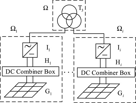
FIGURE 1. Schematic diagram of the association set.
Failure Correlation Analysis
In this study, the decision-making experiment analysis method (DEMATEL) is combined with the interpretation structure model method (ISM) to describe the failure propagation process between the components of the photovoltaic power generation system. Specific ideas are shown in Figure 2. The specific steps are as follows:
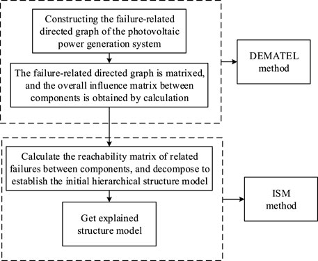
FIGURE 2. Block diagram of failure correlation.
Establishing a Directed Graph of System Failures
A photovoltaic power generation system is taken as an example that exists between two parallel subsystems. The failure correlation between components is analyzed through relevant data to obtain a directed graph of photovoltaic power generation system failures, as shown in Figure 3. If the failure of component i in the system causes the failure of component j, there is a directed edge from node i to j.
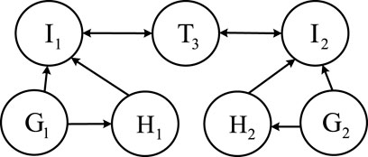
FIGURE 3. Failure directed graph of the photovoltaic power generation system.
Transforming the Directed Graph Into a Matrix and Calculating the Influence Matrix Between the Components
Transforming the invalid and directed graph in Figure 3 into a matrix to obtain the direct influence relationship matrix
where
where
that is,
where
that is,
The reachable matrix
where
The level division table is listed in Table 1 according to the ISM method combined with the reachable matrix.
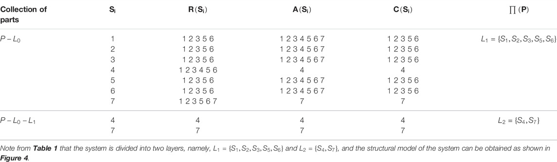
TABLE 1. Process table of level division.
In Table 1,
It can be seen from Figure 4 that the photovoltaic power generation system has a two-level hierarchical structure, and the second level affects the first level, which ultimately affects the development of system reliability. Among them,
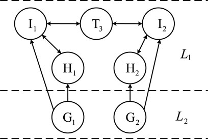
FIGURE 4. Model diagram of the system structure.
Availability Model
Availability Model of Failure-Independent Failure Source Equipment
The equipment in the photovoltaic power generation system age during use, and there are also sudden failures during actual operation. Such failures are usually caused by external random factors that affect the results of maintenance decisions.
According to the IEEE Standard Guide, the operating status of power equipment is divided into normal, attention, abnormal, and serious status (IEEE, 2008). In the traditional status transition model, the serious status is generally treated as failure. In order to comprehensively consider the degraded faults and sudden faults, this study distinguishes the serious status from the faulty status and establishes an improved Markov status transition model to describe the fault law of the equipment.
Figure 5 shows the process of equipment state transition. In the figure, 0–3 indicate normal, attention, abnormal, and degraded failure states; 4–6 denote sudden failure states. It is to be noted that the transfer rate between states is marked in the figure. In addition,
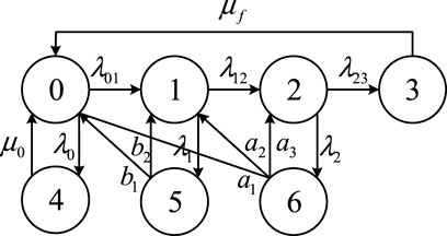
FIGURE 5. Process of equipment state transition.
Assuming that the initial state of the device is 0, the Markov state transition rate matrix of the device based on the aforementioned analysis is as follows:
where
Carrying out the Laplace transform on the aforementioned formula, we obtain:
Obtaining
Availability Model of Nonfailure Source Equipment Considering Failure Correlation
When there is a failure correlation between equipment
where
It can be obtained that the comprehensive failure rate of components is as follows:
where
The Copula theory connects the joint and marginal distribution functions and can systematically describe the correlation characteristics between variables. Therefore, this study proposes the use of this theory and Sklar theorem to obtain the correlation coefficient of the actual degradation. Through the aforementioned analysis combined with the description of the availability model in Fig 3.1, the availability model of nonfailure source equipment that considers the failure correlation can be obtained.
System Availability Model
To compare the availability of photovoltaic power generation systems with and without failure correlation, this section analyzes the system availability model from the point of view of the following two aspects:
Failure-Independent System Availability Model
It is to be noted from the structural analysis of the photovoltaic power generation system in Structural Correlation Analysis that the photovoltaic power generation system unit comprises two subsystems
where
FIGURE 6. Process of subsystem state transition.
In Figure 6, 0 represents the operating status of the subsystem.
Given that the state transition rate of the subsystem is constant, its transition can be described by a Markov process, and the transition rate matrix can be obtained as follows:
From the aforementioned formula, the following C–K equation can be obtained:
where
Then, the availability of subsystem
Accordingly, the overall availability of the photovoltaic power generation unit system can be obtained as follows:
Failure-Related System Availability Model
Based on the description in Availability Model, applying the availability model of nonfailure source equipment to the failure-independent system availability model can obtain a system availability model considering failure correlation.
Photovoltaic Power Generation System Maintenance Model Considering Component Relevance and Availability
Maintenance-Model Thinking Framework
The operation and maintenance of photovoltaic power generation systems must keep the lowest maintenance cost under certain availability conditions. Therefore, upper and lower optimization models are proposed.
The upper model considers the economic structure relevance, introduces the idea of opportunistic maintenance in the modeling process, and determines the maintenance method, time, and scope with the lowest maintenance cost as the objective function. The lower model is a verification based on the upper model, with the highest system availability as the objective function. The component availability is the constraint, and the maintenance plan that does not satisfy the lower model is substituted into the upper layer and optimized again until the optimal maintenance plan is obtained. In this study, the quantum genetic optimization algorithm is proposed to optimize the upper and lower models. A block diagram is shown in Figure 7.
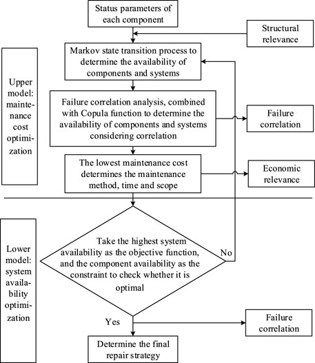
FIGURE 7. Framework of the maintenance model.
Upper-Level Optimization Model
This study takes the lowest maintenance cost in the entire maintenance time period as the objective function and establishes the upper-level optimization model with maintenance resources and time as constraints.
The total maintenance cost of a photovoltaic power station comprises fixed maintenance cost
where
Fixed Cost of Maintenance
The fixed cost of maintenance is determined by the maintenance method, that is, the action set = {minor repair, incomplete maintenance, overhaul} = {0,1,2}. The corresponding maintenance cost is
where
Shutdown Loss
The traditional photovoltaic power plant maintenance model ignores the impact of different weather conditions (irradiance, temperature, etc.) on the shutdown loss and sets the shutdown loss to a fixed value that cannot effectively reflect the actual photovoltaic power station loss. Therefore, in this study, the capacity factor
where
where
where
where
where
Maintenance Personnel Cost
Maintenance personnel expenses include basic salary and bonus:
where
Constraints
Constraints on Maintenance Resources
During the overhaul period, owing to resource constraints such as manpower and required materials, the equipment cannot be simultaneously overhauled. It needs to be performed in sequence. Therefore, there is
where
Constraint on Maintenance Time
The overhaul time is limited to the time period that can be overhauled.
where
Lower-Level Optimization Model
In the upper layer, the maintenance plan obtained with the lowest maintenance cost is brought to the lower layer for verification. The target is the highest availability of the photovoltaic power generation system, and the component availability is the constraint to establish the lower-layer optimization model expressed as follows:
where
where l is the maintenance cost’s adjustment parameter, b is the maintenance frequency’s adjustment parameter, and i is the maintenance frequency. l and b are considered to be 1 and 0.0005, respectively.
Simulation Analysis
In this study, using MATLAB software, taking a 10-MW photovoltaic power station as an example, the economic effectiveness of the model is verified by simulation. According to relevant data of the power station and previous studies, the device state transfer rate can be calculated as shown in Table 2, where the sudden failure rate is set as
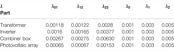
TABLE 2. State transition rate of different devices.
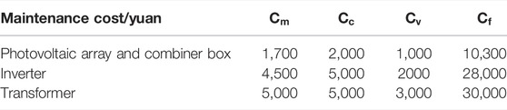
TABLE 3. Maintenance costs of different maintenance methods.
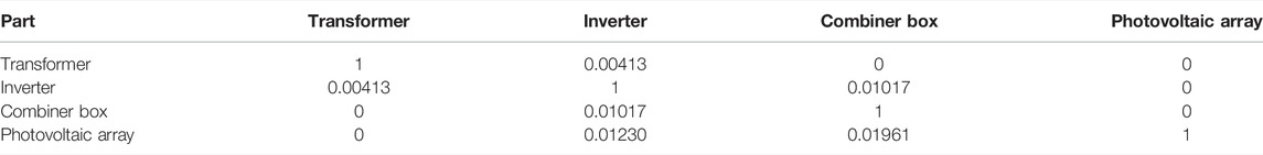
TABLE 4. Correlation coefficient of the actual degradation.
Figure 8 shows the monthly weather accessibility and capacity factor based on the environment where the photovoltaic power station is located and also weather station data.
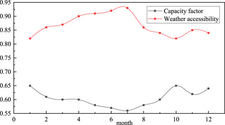
FIGURE 8. Weather parameters.
Performance Comparison Analysis
Two options were selected for comparison analysis.
Option 1: performance analysis without considering the failure correlation. option 2: performance analysis including the failure correlation.
Through the simulation, In Figures 9A,B are shown, respectively, the availability comparison curves of the combiner box and the system under the failure-related strength
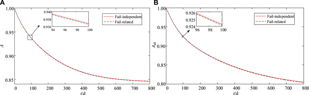
FIGURE 9. Comparison curve of system availability. (A) Comparison curve of availability about
It can be seen from Figure 9 that when the failure correlation is considered, the degree of decline in the availability of equipment and systems increases. It is determined by the correlation coefficient and strength between its increasing speed and equipment. The larger the correlation coefficient, the faster the availability curve of option 2 declines than that of option 1. It can be seen that ignoring the failure correlation will lead to errors in subsequent maintenance strategies and time, thus affecting the revenue of the photovoltaic power generation system.
In order to compare the effects of different failure-related strengths on the availability of equipment and systems, the availability simulation curves are obtained by setting different failure-related strengths as shown in Figure 10.
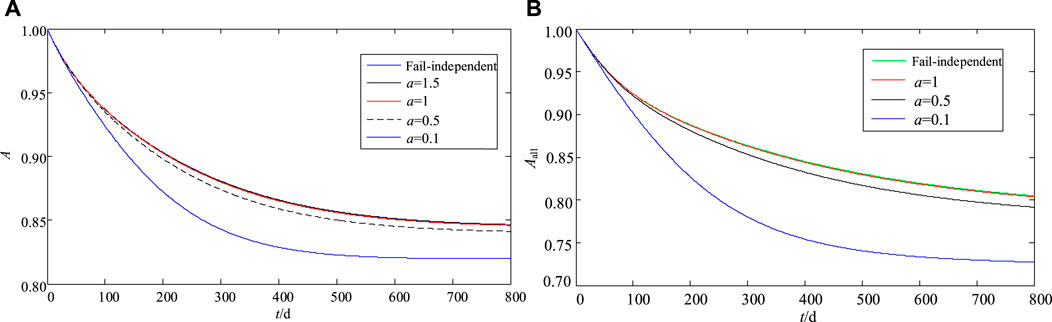
FIGURE 10. Availability curves for different failure-related strengths. (A) Availability curve of the combiner box with different failure-related strengths. (B) Availability curve of the system with different failure-related strengths.
It can be seen from Figure 10 that the failure-independent availability curve is always above the failure-related availability curve, and when the failure-related strength is greater, the availability curve is closer to the failure-independent curve.
When
Comparison of Maintenance Strategies
The following four options are used to compare and analyze: Option 1: a double-layer optimization maintenance strategy that considers component relevance and
The following results were obtained through the simulation analysis: A and B in Figure 11 are the comparison diagrams of the changeable curves of the availability of the combiner box
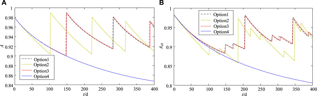
FIGURE 11. Comparison curve of availability after maintenance. (A) Comparison curve of availability of
It can be seen from A in Figure 13 that the availability of the combiner box
B in Figure 13 is the curve of availability change after system maintenance. If the failure correlation is not considered, the transformer needs to be repaired when the system runs to the 206th and 34th days. If the failure correlation is considered, the transformer needs to be repaired when the system runs to the 186th and 34th days, and the system availability is significantly improved after repair.
It can be seen from Figure 11 that the availability of the double-layer optimization maintenance model is significantly improved compared with that of the traditional condition maintenance model. The maintenance time of the double-layer optimization maintenance model considering failure correlation is earlier than that of the double-layer optimization maintenance model with independent failure, and the smaller the value of a, the longer the maintenance time in advance.
Table 5 shows the common maintenance time decision set for photovoltaic power generation unit systems.
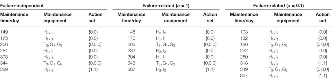
TABLE 5. Maintenance decision set.
It can be seen from the table that the maintenance strategy of failure-independent system and the maintenance strategy of failure correlation are different. When the failure-related strength a is smaller, the maintenance time is earlier; the maintenance times are greater in number in the whole maintenance cycle, and the maintenance cost is higher. This is because when the failure correlation is considered, the probability of failure of the affected component will increase, so the number of repairs will increase, the maintenance cost will increase, and the maintenance strategy will also change. When the failure-related strength
The total maintenance cost of each equipment is calculated by formulas (19–26), resulting in 66,800 yuan, whereas the maintenance cost is 59,200 yuan after adopting the double-layer optimization model. The saving rate reaches 12.8%, and the downtime of each equipment is 72 h for individual maintenance. The double-layer optimization maintenance model that considers opportunistic maintenance takes into account multiple maintenance equipment. The longest maintenance equipment downtime is taken as the common downtime, which is 40 h. As a result, the downtime saving rate can reach 44.4%, so the double-layer optimization model proposed in this study can effectively reduce both downtime and maintenance costs.
Sensitivity Analysis
The double-layer optimization maintenance strategy proposed in this study is affected by weather accessibility. The maintenance-cost change rate and system availability are different under different values.
Impact of Weather Accessibility on the Change Rate of Maintenance Costs
The following two options are used to compare and analyze the influence of weather accessibility on the change rate of maintenance costs:
Option 1: a double-layer optimization maintenance model considering component relevance;
Option 2: traditional condition maintenance model
Figure 12 shows that as the weather accessibility increases, the maintenance shutdown loss decreases, and the reduction rate of the maintenance-cost change-rate decreases. The maintenance-cost saving rate of option 1 is lower than that of option 2. The reason is that the larger the weather accessibility, the smaller the shutdown loss, and the smaller the maintenance-cost saving rate. When
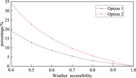
FIGURE 12. Change rate curve of maintenance cost.
Impact of Weather Accessibility on System Availability
Figure 13 shows the impact of the double-layer optimization maintenance model on the availability of photovoltaic power generation systems under different weather accessibility. As shown in the figure, the lower the weather accessibility, the greater the reduction ratio of the system availability. The system reduction ratio presents a normal fluctuation state within 400 days and peaks in the third and sixth maintenance occurrences. This is related to the time required for maintenance of the transformer. It can be seen that under the condition of low access rate, ignoring the weather factor has a greater impact on the maintenance strategy.
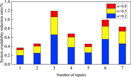
FIGURE 13. Impact of different weather accessibility on system availability.
Conclusion
This study considered the influence of component correlation on maintenance time and strategy and proposed a double-layer optimization maintenance strategy for photovoltaic power generation systems based on component correlation. The following conclusions were obtained through simulation:
By analyzing the failure correlation between components, a multilevel hierarchical structure model of the photovoltaic power generation system was obtained, which interpreted the failure transmission process of the system.
Through the establishment of upper and lower optimization models, the best maintenance time and strategy were obtained by comprehensively considering maintenance costs and optimal availability, thereby effectively reducing maintenance costs, reducing downtime, and improving system availability.
When the failure correlation is considered, the more the maintenance times of the affected components, the higher the maintenance cost, and the maintenance strategy is different from the maintenance model that does not consider failure correlation.
The effect of failure correlation on the availability of equipment and systems was verified by setting different failure-related strengths. The results showed that the smaller the failure-related strength, the greater the impact on the availability of system, which in turn affects the maintenance time and the formulation of maintenance strategies.
The influence of weather accessibility on maintenance costs and system availability was analyzed. The results showed that the lower the weather accessibility, the greater the maintenance cost saving rate and the reduction ratio of the system availability of the double-layer optimization maintenance model, which verified the universal applicability of the strategy in complex environments.
This study failed to consider the competitive failure problem of degradation and shock between devices in the research process. Factors such as risk were not taken into account in maintenance modeling, which will be the next step to be carried out in the future.
Data Availability Statement
The original contributions presented in the study are included in the article/Supplementary Material, further inquiries can be directed to the corresponding author.
Author Contributions
WC: direct participation, including obtaining research funding, guiding the content of articles, and reviewing. XL: direct participation, simulation analysis, data collection, manuscript writing, and revision. Others: supporting contribution and material support.
Funding
This work was supported by the National Natural Science Foundation of China (grant number 51767017) and the Basic Research Innovation Group Project of Gansu Province (grant number 18JR3RA133).
Conflict of Interest
The authors declare that the research was conducted in the absence of any commercial or financial relationships that could be construed as a potential conflict of interest.
Publisher’s Note
All claims expressed in this article are solely those of the authors and do not necessarily represent those of their affiliated organizations, or those of the publisher, the editors, and the reviewers. Any product that may be evaluated in this article, or claim that may be made by its manufacturer, is not guaranteed or endorsed by the publisher.
Acknowledgments
The authors are very grateful for the helpful comments from the reviewers.
References
Catelani, M., Ciani, L., and Galar, D. (2020). Optimizing Maintenance Policies for a Yaw System Using Reliability Centered Maintenance and Data-Driven Condition Monitoring[J]. IEEE Trans. Instrumentation Meas. 69 (9), 6241–6249. doi:10.1109/tim.2020.2968160
Colombi Gomes, L., and Rodrigues Muniz, P. (2020). Economic Optimization of Maintenance against Soiling in Photovoltaic Plants. IEEE Latin Am. Trans. 18 (11), 1884–1891. doi:10.1109/TLA.2020.9398629
Fu, Y., Fan, Y., and Liu, L. (2019). Preventive Maintenance Strategy for Offshore Wind Turbines Considering Component Correlation[J]. PowerSystem Tech. 43 (11), 4057–4063.
Gunda, T., Hackett, S., Kraus, L., Downs, C., Jones, R., McNalley, C., et al. (2020). A Machine Learning Evaluation of Maintenance Records for Common Failure Modes in PV Inverters. IEEE Access 8, 211610–211620. doi:10.1109/ACCESS.2020.3039182
IEEE B. E. (2009). IEEE Guide for the Interpretation of Gases Generated in Oil-Immersed Transformers IEEE. doi:10.1109/IEEESTD.2009.4776518
Li, J., Xu, J., and Ren, L. (2021). Incomplete Preventive Replacement and Maintenance Model under Reliability Constraints [J/OL]. Acta Solar Energy 1-7, 05–27. doi:10.19912/j.0254-0096.tynxb.2020-1372
Liu, L., Fu, Y., and Ma, S. (2015). Maintenance Strategy for Offshore Wind Turbines Based on Monitoring and Prediction of Operating Conditions [J]. Power Syst. Tech. 39 (11), 3292–3297.
Mahani, K., Liang, Z., and Parlikad, A. K. (2018). Joint Optimization of Operation and Maintenance Policies for Solar-Powered Microgrids[J]. IEEE Trans. Sust. Energ. 10 (2), 833–842. doi:10.1109/TSTE.2018.2849318
Mengying, H., Jianhua, Y., and Xiao, Z. (2021). Joint Optimization of Inspection, Maintenance, and Spare Ordering Policy Considering Defective Products Loss. J. Syst. Eng. Electron. 32 (5), 1167–1179. doi:10.23919/JSEE.2021.000100
Nguyen, N., Almasabi, S., and Mitra, J. (2019). Impact of Correlation between Wind Speed and Turbine Availability on Wind Farm Reliability. IEEE Trans. Ind. Applicat. 55 (3), 2392–2400. doi:10.1109/TIA.2019.2896152
Oprea, S. V., Bara, A., and Preotescu, D. (2019). Potovoltaic Power Plants (PV-PP) Reliability Indicators for Improving Operation and Maintenance Activities. A Case Study of PV-PP Agigea Located in Romania[J]. IEEE Access 7, 39142–39157. doi:10.1109/access.2019.2907098
Peng, F., Yu, H., Tao, J., Su, Y., Zhou, D., Zeng, X., et al. (2020). Efficient Statistical Analysis for Correlated Rare Failure Events via Asymptotic Probability Approximation. IEEE Trans. Comput.-Aided Des. Integr. Circuits Syst. 39 (12), 4971–4984. doi:10.1109/TCAD.2020.2979804
Perdue, M., and Gottschalg, R. (2015). Energy Yields of Small Grid Connected Photovoltaic System: Effects of Component Reliability and Maintenance. IET Renew. Power Generation 9 (5), 432–437. doi:10.1049/iet-rpg.2014.0389
Song, S., Coit, D. W., Feng, Q., and Peng, H. (2014). Reliability Analysis for Multi-Component Systems Subject to Multiple Dependent Competing Failure Processes. IEEE Trans. Rel. 63 (1), 331–345. doi:10.1109/TR.2014.2299693
Spertino, F., Chiodo, E., and Ciocia, A. (2021). Maintenance Activity, Reliability, Availability and Related Energy Losses in Ten Operating Photovoltaic Systems up to 1.8 MW[J]. IEEE Trans. Industry Appl. 57 (1), 83–93. doi:10.1109/tia.2020.3031547
Sun, Y., and Sun, Z. (2021). Selective Maintenance on a Multi-State Transportation System Considering Maintenance Sequence Arrangement[J]. IEEE Access 9, 70048-70060. doi:10.1109/access.2021.3078140
Verbert, K., De Schutter, B., and Babuška, R. (2017). Timely Condition-Based Maintenance Planning for Multi-Component Systems. Reliability Eng. Syst. Saf. 159, 310–321. doi:10.1016/j.ress.2016.10.032
Wang, Q., He, Z., Lin, S., and Liu, Y. (2018). Availability and Maintenance Modeling for GIS Equipment Served in High-Speed Railway under Incomplete Maintenance. IEEE Trans. Power Deliv. 33 (5), 2143–2151. doi:10.1109/TPWRD.2017.2762367
Xu, A. S., Gebraeel, N. Z., and Yildirim, M. (2017). Integrated Predictive Analytics and Optimization for Wind Farm Maintenance and Operations[J]. IEEE Trans. Power Syst. 138:110639 doi:10.1016/j.rser.2020.110639
Xu, B., Han, X., and Liu, C. (2015). Decision-making Modelfor System State Maintenance Based on Correlation Set Decomposition[J]. Automation of Electric PowerSystems 39 (02), 46–52. doi:10.7500/AEPS20130906018
Xu, J., Wu, W., Wang, K., and Li, G. (2020). C-vine Pair Copula Based Wind Power Correlation Modelling in Probabilistic Small Signal Stability Analysis. Ieee/caa J. Autom. Sinica 7 (4), 1154–1160. doi:10.1109/JAS.2020.1003267
Zhao, H., Zhang, J., and Cheng, L. (2016). State of Wind Turbines Considering Incomplete Maintenance-Opportunistic Maintenance Strategy[J]. Proc. Chin. Soc. Electr. Eng. 36 (03), 701–708.
Zhu, X., and Liu, Y. (2020). Maintenance Strategy of Photovoltaic Power Plant Based on Component-System Hierarchical Optimization[J]. Automation Electric Power Syst. 44 (08), 92–99. doi:10.7500/AEPS20190626009
[ad_2]