Analysis of Potential Water Inflow Rates at an Underground Coal Mine Using a WOA-CNN-SVM Approach

By inergency On Mar 9, 2024

[ad_1]

1. Introduction

Coal resources occupy a dominant position in China’s energy structure [1], and its demand is huge [2]. With the increasing mining scale and intensity, the problem of coal seam roof water disasters has become increasingly prominent, which seriously threatens the safe mining of coal mines, resulting in surface subsidence and affecting the stability of buildings [3,4]. However, the water yield of aquifers directly affects the occurrence and frequency of water inflow [5]. Moreover, due to the influence of coal seam mining, the water yield of aquifers changes dynamically, and the borehole data are scarce and cannot be characterized globally in space [6]. Therefore, it is of great practical significance to do a good job in predicting roof water yield to reduce water inflow accidents and ensure coal mine safety in production.

Traditional aquifer water yield prediction methods mainly use the analytic hierarchy process (AHP) [7,8], entropy weight method [9], technique for order preference by similarity to an ideal solution (TOPSIS) [10,11], and other analytical methods to construct the weighting matrix and draw the water yield partition, but their shortcomings such as strong subjectivity, weak correlation between the indicators, and strong dependence on the weighting matrix lead to the low accuracy of model prediction. With the development of artificial intelligence, machine learning and neural networks are widely used in different fields [12,13,14,15], and in recent years, they have been gradually applied to the prediction of water yield. According to the water yield characteristics of coal seam roofs, many scholars have proposed a variety of prediction and evaluation methods from different perspectives. Cheng et al. [16] used a bat algorithm to optimize the backpropagation (BP) neural network to realize a quantitative prediction of the water yield of rock strata. Ma et al. [17] proposed a genetic algorithm to optimize a nonlinear gray Bernoulli model for predicting the risk of surge water. Wu et al. [18] proposed a method for assessing the probability of occurrence of mine water emergencies based on the combination of scenario analysis and Bayesian networks. Qu et al. [19] used the information theoretic learning and VlseKriterijuska Optimizacija I Komoromisno Resenje (ITL-VIKOR) method with triangular fuzzy number extension to establish a binary semantic evaluation mathematical model for water yield. Mulumba et al. [20] developed a safety risk assessment model for underground coal mines based on particle swarm optimization and backpropagation (PSO-BP) neural networks. Gul et al. [21] proposed a safety risk assessment method based on Pythagorean fuzzy VIKOR. Mishra et al. [22] used the Bayesian network for risk assessment of roof collapse. The above studies provide new methods for the prediction of aquifer water yield, but the number of samples required is large, which prevents fast and accurate prediction of water yield. Therefore, this paper proposes a model based on WOA-CNN-SVM to improve the prediction accuracy.

The WOA-CNN-SVM prediction model is constructed by selecting multifactor evaluation indexes based on coal mine geological data, which can efficiently predict aquifer water yield with small samples. Compared with other models, this model has higher evaluation accuracy. It can be used to predict the water yield of an area in the absence of unit water inflow rate data and can more accurately portray the spatial dynamic characteristics of water yield.

2. Overview of Baodian Coal Mine

The study area is located in the Jining City area, Shandong Province, and the stratigraphy from top to bottom is Quaternary (Q), Jurassic, (J), Permian (P), Carboniferous (C), and Ordovician (O). The total thickness of the Quaternary layer, composed of brownish yellow, gray-green to gray-white clay, sandy clay, clayey sand (gravel), and sand and gravel layers, is 110~228 m, with an average thickness of 171 m, thin in the southeast and thick in the northwest, and divided into the upper, middle, and lower groups, with average thicknesses of 59 m, 67 m, and 41 m, respectively. The water-bearing layer and water-isolating layer are interlaced with each other, the lenticular body is relatively developed, and the lithology is complicated. The main aquifer is the water-yielding layers of the lower group of sand and gravel layers, which are mainly distributed in the middle, western, and middle-north part of the coal field and are missing in the southeast part of the coal field, which is mainly the alluvial flood layer.

The coal field in the study area belongs to the simple tectonic type. The southern flank is cut by the Huangfu fault, while the northern flank is relatively intact. The stratigraphy of the coal field is undulating, and the folds are characterized by wide and slow short-axis dips, with dips ranging from 2° to 13°, and the dips only vary greatly in local areas (up to 27°). Except for the southern boundary fault (Huangfu fault), the southwestern boundary fault (Majialou fault), and the Puzi fault in the northern part of the coal field, the other faults all have a drop of less than 30 m.

The surface river, Sihe, flows from the western part of the coal field and flows through the upper part of the five mining areas, with a total length of 159 km, a watershed area of 2357 km², a riverbed width of 100~1000 m, and a maximum flow rate of 4020 m³/s. The Sihe River is seasonal, and it also has a certain hydraulic connection with the Quaternary layer. An outline of the coal mine area is shown in Figure 1.

3. Determination of the Main Controlling Factors of Water Inflow

The measurement of water content depends on the unit water inflow rate, and the lack of data makes it impossible to describe the water yield globally. Therefore, by analyzing the influencing factors of water yield, the water yield prediction model is established. Through training the existing data, the results are compared with the actual aquifer pumping test results, which can effectively evaluate the water yield degree of mines lacking the actual inflow data.

Based on the reports of hydrogeological data from 2019 to 2023 by Baodian Coal Mine, such as raising the upper mining limit and the Quaternary aquifer water-yield property research report, private data on hydrology and geology are used to guide coal mine production, and considering the factors affecting water yield of the aquifer and other scholars’ [23,24,25] experience in index selection, six factors are selected from the aspects of hydraulic connection characteristics and aquifer lithology, including aquifer thickness (X₁), radius of influence (based on the drilling diameter of 91 mm and the pumping water level drop of 10 m) (X₂), normalized drawdown (X₃), permeability coefficient (X₄), core recovery percentage (X₅), and the proportion of clay thickness to lower layer thickness (X₆). The thematic map of evaluation indicators is shown in Figure 2.

The thickness of the aquifer is the basis for determining the strength of water yield and is also a direct influence [5]. The greater the thickness of the aquifer, the stronger the water yield. The coefficient of permeability is a quantitative index characterizing the permeability properties of rocks and is positively correlated with water yield. The size of the radius of influence is related to the permeability coefficient of the aquifer and the normalized drawdown. The larger the permeability coefficient of the aquifer is, the larger the normalized drawdown and radius of influence are, and the higher the water yield of the rock is. The core recovery percentage reflects the degree of rock fragmentation. The lower the core take rate is, the better the rock fracture that is developed. The water yield of the bedrock aquifer with coarse and large fissures is better than that of the bedrock drilling with weak fissure development, and vice versa, with a weak water yield, the core recovery percentage has a negative correlation to the water yield and a negative influence on the water yield. The permeability coefficient of the clay layer is smaller than that of the sand layer. The greater the thickness of the clay layer accounting for the thickness of the lower group of Quaternary layers, the smaller its permeability coefficient is and the weaker the aquifer’s ability to produce water, and it shows a negative correlation to the aquifer’s water yield.

4. Composite Modeling Framework

4.1. Convolutional Neural Network Modeling Framework

A convolutional neural network (CNN) is a feed-forward neural network [26] that includes an input layer, a convolutional layer, a pooling layer, a fully connected layer, and an output layer [27,28]. The structure of a traditional CNN model is schematically shown in Figure 3.

The input layer is the first layer of the model, where the image input is passed into the convolutional layer with feature extraction. The convolutional layer is the basis of the model, and the convolutional kernel moves a sliding window over the input image parameters during the established quantization step, thus extracting the feature parameters [29]. After that, the extracted features are fed into the pooling layer, which effectively reduces the redundancy of the information and prevents overfitting [30]. The fully connected layer is connected to the output layer to convert the filtered image into the labeled categories [31].

4.2. Support Vector Machine Model

Support vector machine (SVM) transforms complex low-dimensional nonlinear regression problems into high-dimensional linear regression problems via a nonlinear mapping function

Φ (x)

[32,33] and constructing the regression function as [34]:

$f (x) = ω^{T} \cdot Φ (x) + b$

(1)

where: $ω$ is the high-dimensional feature space; $Φ (x)$ is the nonlinear mapping; $b$ is the threshold value.

The above problem is equivalent to the following optimization [34]:

$\{\begin{cases} \min [\frac{1}{2} {‖ω‖}^{2} + c \sum_{i = 1}^{n} (ξ_{i} + ξ_{i}^{*})] \\ f (x_{i}) - y_{i} \leq ε + ξ_{i} \\ y_{i} - f (x_{i}) \leq ε + ξ_{i}^{*} \end{cases}$

(2)

where: $ξ_{i}$ and $ξ_{i}^{*}$ are relaxation factors; $ε$ is the insensitivity loss factor; $c$ is the penalty factor; $y_{i}$ is the corresponding output of $x_{i}$ .

The regression function can be obtained by introducing the Lagrangian method of solving and transforming the original problem into a pairwise problem [34]:

$f (x) = \sum_{i = 1}^{n} (α_{i}^{*} - α_{i}) k (x, x_{i}) + b$

(3)

where: $α_{i}$ and $α_{i}^{*}$ is Lagrange operator; $k (x, x_{i})$ is the kernel function.

The convolutional neural network part is designed with convolutional layer–BN layer–activation layer–discard layer–fully connected layer structure. The traditional CNN pooling layer achieves dimensionality reduction for high-dimensional redundant data [35], while water yield features have low dimensionality compared to image pixels. Using the pooling layer results in the loss of information [36], so it is not necessary to use the pooling layer stacked into the model structure. Batch normalization can speed up convergence without losing data features [37], the activation layer improves convergence and prevents overfitting [38], and the drop layer enhances the generalization of the model [39].

SVM has the advantages of strong generalization ability and fast computation speed [40] and is good at solving nonlinear classification problems. SVM is used to replace the traditional classifier of the CNN to obtain good prediction performance. The flowchart of the CNN-SVM algorithm is shown in Figure 4.

The prediction steps of the CNN-SVM model are: (1) normalize the data to eliminate the effect of magnitude, divided into a training set and test set, to comply with the model’s need to preprocess the data by tiling; (2) input the training set to the CNN model for training and select the ReLU function as the activation function to achieve the convergence effect and save it; (3) use CNN-extracted feature vectors as the input to the SVM classifier to continue to train; (4) substitution of the test set into the trained model outputs the water yield prediction results and measurement of the accuracy of the predictive model by the prediction results and comparison with the real value.

4.3. Whale Optimization Algorithm

Whale optimization (WOA) [41] is a nature-inspired meta-heuristic optimization algorithm proposed by Seyedali Mirjalili in 2016, which is inspired by the humpback whale bubble-net hunting strategy. Humpback whales can identify the position of prey and surround them. According to their hunting characteristics, three behaviors are abstracted: surround prey, predation, and random search [42].

(1) Surrounding the prey. This behavior is represented by the following equation [41]:

$\{\begin{cases} D = | C \cdot X^{*} (t) - X (t) | \\ X (t + 1) = X^{*} (t) - A \cdot D \end{cases}$

(4)

where: $D$ is the distance between the search agent and the prey; $A$ and $C$ are the coefficient vectors; $X^{*}$ is the position vector of the global optimal solution, updated in each iteration; $X$ is the position vector; and $t$ denotes the number of current iterations.

The equations for the coefficient vectors

A

and

C

are as follows [41]:

$\{\begin{cases} A = 2 a \cdot r_{1} - a \\ C = 2 r_{2} \end{cases}$

(5)

where: $a$ is the convergence factor, which decreases linearly from 2 to 0 during the iteration; $r_{1}$ , $r_{2}$ is a random vector distributed between [0, 1].

(2) Prey predation. Humpback whales attack their prey with a bubble-net strategy, describing the predation behavior designed with both a constricting envelope mechanism and a spiral to update the position. Both occur simultaneously and the mathematical expression is [41]:

$X (t + 1) = \{\begin{cases} X^{*} (t) - A \cdot D, p < 0.5 \\ X^{*} (t) + D^{'} \cdot e^{b l} \cdot \cos (2 π l), p \geq 0.5 \end{cases}$

(6)

where: $D^{'}$ denotes the best distance obtained; $b$ is a constant defining the shape of the logarithmic spiral; $l$ is a random number in [−1, 1]; $p$ is a random number in [0, 1].

(3) Random search. When the coefficient

| A | < 1

, the whale is inside the envelope and selects the spiral envelope prey. When

| A | \geq 1

, the whale is outside the constricted envelope, at which point a random search is performed; the random search is updated with the following equation [41]:

$X (t + 1) = X_{r a n d} (t) - A \cdot | C \cdot X_{r a n d} (t) - X (t) |$

(7)

where: $X_{r a n d}$ is the randomly selected whale position.

The selection of different parameters has a significant impact on the CNN model performance. To achieve the optimal performance of the model, it is optimized using the whale optimization algorithm. The CNN model optimized by the whale algorithm is constructed. (1) Normalize the data using Formulas (8) and (9) to eliminate the effect of magnitude, set the number of WOA optimization parameters and the upper and lower limits of the optimization objective, initialize the position of the whale population, and search for the optimal results and output them; (2) construct the CNN model according to the optimal results and train the data to obtain the feature parameters; (3) feed the extracted feature parameters into the SVM network to continue to complete the prediction and output the results of the prediction of the water yield. The framework of the WOA-CNN prediction model is shown in Figure 5.

$g_{i} = \frac{G_{i} - \min (G)}{\max (G) - \min (G)}$

(8)

$g_{i} = \frac{\max (G) - G_{i}}{\max (G) - \min (G)}$

(9)

where: $g_{i}$ is the normalized data; $G$ is the original data; $G_{i}$ is the $i$ -th value of the original data.

5. Model Construction and Validation

5.1. Model Construction

China’s “Detailed Rules for Water Prevention and Control in Coal Mines” takes the unit water inflow rate (q) of boreholes as the basis for judging the water content of aquifers. Therefore, the unit water inflow rate was taken as the target value for regression prediction. A nonlinear prediction model based on each characteristic variable and unit water inflow rate was established, and the model was trained and predicted according to the model prediction process in Figure 4 and Figure 5. The relevant parameters of the model were set as follows: the population size of whales in WOA N = 10, and the number of target optimization parameters D = 3. The learning rate, the batch size, and the regularization coefficient [43] were optimized, and their optimization search ranges were [1 × 10⁻³, 1 × 10⁻²], [32, 256], [1 × 10⁻⁴, 1 × 10⁻¹], respectively. The CNN model was optimized for a maximum of 300 iterations, and the learning rate decreased after 240 iterations.

The borehole data in Table 1 are substituted into the established WOA-CNN-SVM prediction model. Eighty percent of the data are used as training samples for model training, and the remaining data are used as test samples to check the model prediction accuracy. The loss function is used to record the degree of matching between predicted and true values [37] and, as shown in Figure 6a, it can be seen that the function decreases sharply in the early stages and gets closer to the true values and tends to be stabilized after the 150th iteration, indicating that the model converges on the training set. The optimal parameter combination is 0.0037 for the learning rate, 87 for the batch size, and 0.0001 for the regularization factor.

The prediction results of the samples in the training set and test set are shown in Figure 6b,c. It can be seen that the predicted values are basically in line with the real values.

Two indicators, root mean square error (RMSE) and mean absolute error (MAE), are usually used to evaluate the performance of each model [44,45]. Smaller RMSE and MAE indicate more accurate prediction results. Their calculation formulas are as follows:

$\{\begin{cases} RMSE = \sqrt{\frac{\sum_{i = 1}^{N} {(Y_{i} - y_{i})}^{2}}{N}} \\ MAE = \frac{1}{N} \sum_{i = 1}^{N} | Y_{i} - y_{i} | \end{cases}$

(10)

where: $N$ is the number of samples; $Y_{i}$ is the true value; $y_{i}$ is the predicted value.

The RMSE of the training set and test set are 0.0269 and 0.0318, respectively. The MAE is 0.0125 and 0.0268, respectively, which is a good prediction effect, and there is no overfitting phenomenon. The model can be applied to the prediction of water yield.

5.2. Model Prediction Performance Testing

To test the effectiveness of the model optimization results, the same set of borehole data is used as training and testing samples, and the unoptimized machine learning models SVM, CNN, WOA-SVM, WOA-CNN, and CNN-SVM are selected for comparison.

The parameter settings of each model are as follows: 2 CNN hidden layers, 300 iterations, 0.01 learning rate, and 0.3 discarded layers. The penalty factor c and kernel function parameter g of the SVM model are 4.5 and 0.6, respectively [46]. To control the variables, the parameter settings mentioned before are used for all models.

To obtain a more intuitive picture of the difference between the predicted and true values of each model, a line graph of the predicted and true values of each model is plotted. As shown in Figure 7. The higher the overlap between the two, the more accurate the model prediction.

It can be seen from Figure 7 that the predicted value and the real value of the WOA-CNN-SVM model match to the highest degree. The CNN model has the worst prediction effect, and the correct rate is increased by 5.88% after combining with the SVM model, which shows that the generalization ability of regression prediction by the SVM classifier is improved. However, there are errors in the 11th, 16th, and 20th samples, because the characteristic data are similar and errors easily occur in the prediction. The accuracy of SVM and CNN models optimized by the whale algorithm is improved by 22.73% and 5.88%, respectively, which shows that the whale optimization algorithm plays an active role in improving the accuracy.

To ensure the reliability of the results, multiple runs were averaged. The prediction performance of each model is presented in Figure 8a. The WOA-CNN-SVM model exhibits the highest and most stable prediction accuracy, with RMSE and MAE values of 0.0318 and 0.0268, respectively. The predictions of the unoptimized model deviated more compared to the true values. The optimized composite model matched the true values to the highest degree, with a correct rate of around 92%. The results show that the optimized model has better prediction performance and is closer to the true value.

In addition, the optimized composite model is compared with other types of commonly used models, such as a BP neural network, random forest (RF) network, and long short-term memory (LSTM) network. Among them, the relevant parameter settings of the BP neural network and long short-term memory network are the same as those of the CNN mentioned earlier, the number of decision trees in the random forest network is 300, and the minimum number of leaves is 2. The prediction performance results of each model after training are shown in Figure 8b.

The composite model showed high performance, followed by random forest networks. The BP neural network exhibits less stable predictive performance. These results indicate that the automatically learned data features of the water yield prediction model based on WOA-CNN-SVM can more effectively characterize the mapping relationship between the unit water inflow rate and the influencing factors, thus obtaining a higher prediction accuracy.

6. Discussion

6.1. Water Yield Zoning Predictions

Substituting the borehole data lacking the unit water inflow rate into the model, the predicted unit water inflow rate was obtained in the range of 0.00003~0.5293 L/(s·m), and the results of the borehole predictions are shown in Table 2.

Based on the WOA-CNN-SVM prediction results, the unit water inflow rate is interpolated by inverse distance weight using a GIS spatial drawing tool to realize the visualization of water yield areas. To obtain a 3D surface map, the interpolation data are exported by Surfer software(Surfer 15)and then depicted by the Origin drawing tool, as shown in Figure 9.

Figure 9a is classified according to the provisions of the water control regulations and can be used to verify the correctness of the predicted results. According to all the predicted results, it can be seen that there is no very strong water yield, so it is divided into three class areas. According to the hydrological records of the fourth system, the unit water inflow rate of borehole 2009-1 is 0.539 L/(s·m), which belongs to the moderately transmissive zone, while the unit water inflow rate of borehole 2010-3 is 0.00008 L/(s·m), which indicates a very poor transmissive zone. This classification result is consistent with the actual degree of water yield. Other drill holes were similarly validated, with up to 97.56% correct water yield zoning based on a comparison of known results.

However, due to the wide-area-oriented nature of the water control regulations, they are generalized and lack the refinement of zoning. The refinement of water yield is also carried out, and the division results are relative to the entire interior of the mine area. Figure 9b,c shows that the eastern and southern parts of the study area generally have a weak water yield, while the western and northern parts have more water yield. This pattern can be attributed to the fact that the thickness of the Lower Quaternary strata in the western part of the coal field in the fifth and sixth mining zones ranges from 14 m to 57 m, with an average of 40 m. The aquifers gradually develop from the south to the north, showing the characteristics of thinness in the south and thickness in the middle and the north. In addition, the aquifer in the lower part of the Quaternary system and the water separation layer in the coal field of the southern eight mining areas are relatively stable, effectively blocking the hydraulic connection. Therefore, the recharge conditions of the lower aquifer are poor and the water yield is relatively weak. The zoning of strong and weak water yield is generally in line with the actual situation of the mining area. The inspection of the stronger zones can be appropriately strengthened to avoid the formation of water-conducting channels due to mining disturbance.

6.2. Strengths and Limitations

The important achievement of this study is to put forward a compound prediction model, which can provide a new idea for readers to accurately and reliably evaluate the water yield of aquifers in mining areas to guide coal mining. The limited borehole data and dimensions of main control factors may be the main reason for the error between the predicted results and the actual values. In the future, we can rely on the advantages of big data to realize data sharing and make the model more suitable for water yield prediction through more data training.

7. Conclusions

In order to investigate the water yield of aquifers that pose a threat to coal mine safety production, the water yield in the study area was predicted and categorized based on mine borehole exploration data using the WOA-CNN-SVM prediction model, with a representative coal mine selected. The main conclusions are as follows:

(1): The combination of CNN and SVM models improves the correct rate of prediction results by about 24%, showcasing strong generalization ability. In addition, after applying the whale optimization algorithm, the prediction correctness is significantly improved. The whale optimization algorithm demonstrated remarkable global search ability, preventing it from becoming trapped in local optima and enhancing the accuracy of water yield prediction. Additionally, it overcame the issue of requiring a large number of samples in traditional methods and effectively addressed data scarcity caused by a limited number of pumping holes. Therefore, it proved feasible to predict water yield levels.
(2): A multifactor composite water yield prediction model for aquifers was developed, using aquifer thickness, influence radius, water level drop, permeability coefficient, borehole coring rate, and the ratio of clay thickness to the lower group thickness as evaluation criteria. Compared with the unoptimized model and other models, the WOA-CNN-SVM model has significantly lower root mean square error and mean absolute error.
(3): Based on the validation of the provisions of the water control regulations, the predictions are in accordance with the regulations. It also carries out the delineation of water yield areas relative to the interior of the mine. The northern part of the fifth mining area and the north-central part of the sixth mining area in the study area displayed relatively strong water yield, with well-developed aquifers in the northern section. Conversely, the southern part of the eighth mining area exhibited generally weak water yield, with the middle group of the Quaternary system well-developed and stable, effectively blocking the hydraulic connection between the upper and lower Quaternary aquifer groups. As a result, the water yield of individual aquifers in that area was moderately weak. Comparisons within the mining region are similarly realistic, signifying the feasibility of the water yield prediction model based on WOA-CNN-SVM.

Author Contributions

W.L.: Investigation, Methodology, Writing—original draft, Writing—review and editing. Y.R.: Data curation, Investigation, Methodology, Project administration, Writing—original draft. X.M.: Investigation, Methodology, Writing—original draft, Writing—review and editing. B.T.: Investigation, Writing—original draft. X.L.: Investigation. All authors have read and agreed to the published version of the manuscript.

Funding

This work was funded by the Natural Science Foundation of Shandong Province (ZR2023ME002) and the SDUST Research Fund (grant 2018TDJH102).

Data Availability Statement

All data analyzed during the study are included in the submitted article.

Conflicts of Interest

Author Bo Tian was employed by the company Shandong Energy Group Co., Ltd. The remaining authors declare that the research was conducted in the absence of any commercial or financial relationships that could be construed as a potential conflict of interest.

References

Wu, Q.; Tu, K.; Zeng, Y.F.; Liu, S.Q. Exploration of the main problems and countermeasures for creating an upgraded version of China’s main energy source (coal). J. China Coal Soc. 2019, 44, 1625–1636. [Google Scholar]
Zeng, Y.; Meng, S.; Wu, Q.; Mei, A.; Bu, W. Ecological water security impact of large coal base development and its protection. J. Hydrol. 2023, 619, 129319. [Google Scholar] [CrossRef]
Zhao, Y.; Wu, Q.; Chen, T.; Zhang, X.; Du, Y.; Yao, Y. Location and flux discrimination of water inrush using its spreading process in underground coal mine. Saf. Sci. 2020, 124, 104566. [Google Scholar] [CrossRef]
Zhang, C.; Jin, Z.; Feng, G.; Song, X.; Rui, G.; Yujiang, Z. Double Peaked Stress–Strain Behavior and Progressive Failure Mechanism of Encased Coal Pillars Under Uniaxial Compression. Rock Mech. Rock Eng. 2020, 53, 3253–3266. [Google Scholar] [CrossRef]
Qiu, M.; Yin, X.; Shi, L.; Zhai, P.; Gai, G.; Shao, Z. Multifactor Prediction of the Water Richness of Coal Roof Aquifers Based on the Combination Weighting Method and TOPSIS Model: A Case Study in the Changcheng No. 1 Coal Mine. ACS Omega 2022, 7, 44984–45003. [Google Scholar] [CrossRef] [PubMed]
Bi, Y.; Wu, J.; Tang, L.; Zhai, X.; Huang, K.; Liu, W. Water Abundance Comprehensive Evaluation of Coal Mine Aquifer Based on Projection Pursuit Model. Lithosphere 2022, 2021, 3259214. [Google Scholar] [CrossRef]
Wang, Q.; Wang, H.; Qi, Z. An application of nonlinear fuzzy analytic hierarchy process in safety evaluation of coal mine. Saf. Sci. 2016, 86, 78–87. [Google Scholar] [CrossRef]
Xu, Y.; Ma, L.; Yu, Y. Water Preservation and Conservation above Coal Mines Using an Innovative Approach: A Case Study. Energies 2020, 13, 2818. [Google Scholar] [CrossRef]
Ma, J.; Dai, H. A methodology to construct warning index system for coal mine safety based on collaborative management. Saf. Sci. 2017, 93, 86–95. [Google Scholar] [CrossRef]
Long, R.; Li, H.; Wu, M.; Li, W. Dynamic evaluation of the green development level of China’s coal-resource-based cities using the TOPSIS method. Resour. Policy. 2021, 74, 102415. [Google Scholar] [CrossRef]
Mahdevari, S.; Shahriar, K.; Esfahanipour, A. Human health and safety risks management in underground coal mines using fuzzy TOPSIS. Sci. Total. Environ. 2014, 488–489, 85–99. [Google Scholar] [CrossRef]
Hwang, S.-H.; Mangalathu, S.; Shin, J.; Jeon, J.-S. Machine learning-based approaches for seismic demand and collapse of ductile reinforced concrete building frames. J. Build. Eng. 2021, 34, 101905. [Google Scholar] [CrossRef]
Luan, L.-T.; Ha, N.-T.-V.; Lee, J.; Nguyen-Xuan, H. Machine learning-based real-time daylight analysis in buildings. J. Build. Eng. 2022, 52, 104374. [Google Scholar]
Zhang, J.; Huang, Y.; Cheng, H.; Chen, H.; Xing, L.; He, Y. Ensemble learning-based approach for residential building heating energy prediction and optimization. J. Build. Eng. 2023, 67, 106051. [Google Scholar] [CrossRef]
Degtyarev, V.V.; Tsavdaridis, K.D. Buckling and ultimate load prediction models for perforated steel beams using machine learning algorithms. J. Build. Eng. 2022, 51, 104316. [Google Scholar] [CrossRef]
Cheng, J.L.; Zhao, J.H.; Dong, Y.; Dong, Q.Y. Quantitative prediction of water abundance in rock mass by transient electro–magnetic method with LBA–BP neural network. J. China Coal Soc. 2020, 45, 330–337. [Google Scholar]
Ma, D.; Bai, H. Groundwater inflow prediction model of karst collapse pillar: A case study for mining-induced groundwater inrush risk. Nat. Hazards 2015, 76, 1319–1334. [Google Scholar] [CrossRef]
Wu, J.; Xu, S.; Zhou, R.; Qin, Y. Scenario analysis of mine water inrush hazard using Bayesian networks. Saf. Sci. 2016, 89, 231–239. [Google Scholar] [CrossRef]
Qu, X.; Han, J.; Shi, L.; Qu, X.; Bilal, A.; Qiu, M.; Gao, W. An extended ITL-VIKOR model using triangular fuzzy numbers for applications to water-richness evaluation. Expert Syst. Appl. 2023, 222, 119793. [Google Scholar] [CrossRef]
Mulumba, D.M.; Liu, J.; Hao, J.; Zheng, Y.; Liu, H. Application of an Optimized PSO-BP Neural Network to the Assessment and Prediction of Underground Coal Mine Safety Risk Factors. Appl. Sci. 2023, 13, 5317. [Google Scholar] [CrossRef]
Gul, M.; Ak, M.F.; Guneri, A.F. Pythagorean fuzzy VIKOR-based approach for safety risk assessment in mine industry. J. Saf. Res. 2019, 69, 135–153. [Google Scholar] [CrossRef]
Mishra, R.; Uotinen, L.; Rinne, M. A Bayesian network approach for geotechnical risk assessment in underground mines. J. South. Afr. Inst. Min. Met. 2021, 121, 287–294. [Google Scholar] [CrossRef]
Wang, S.-S.; Song, B.-L. Application of fuzzy analytic hierarchy process in sandstone aquifer water yield property evaluation. Environ. Technol. Innov. 2021, 22, 101488. [Google Scholar] [CrossRef]
Liu, W.; Zheng, Q.; Pang, L.; Dou, W.; Meng, X. Study of roof water inrush forecasting based on EM-FAHP two-factor model. Math. Biosci. Eng. 2021, 18, 4987–5005. [Google Scholar] [CrossRef] [PubMed]
Sun, Z.; Bao, W.; Li, M. Comprehensive Water Inrush Risk Assessment Method for Coal Seam Roof. Sustainability 2022, 14, 10475. [Google Scholar] [CrossRef]
Li, Z.; Liu, F.; Yang, W.; Peng, S.; Zhou, J. A Survey of Convolutional Neural Networks: Analysis, Applications, and Prospects. IEEE Trans. Neural Netw. Learn. Syst. 2022, 33, 6999–7019. [Google Scholar] [CrossRef]
Sun, Y.; Xue, B.; Zhang, M.; Yen, G.G. Evolving Deep Convolutional Neural Networks for Image Classification. IEEE Trans. Evol. Comput. 2020, 24, 394–407. [Google Scholar] [CrossRef]
Shao, H.; Xia, M.; Han, G.; Zhang, Y.; Wan, J. Intelligent Fault Diagnosis of Rotor-Bearing System Under Varying Working Conditions With Modified Transfer Convolutional Neural Network and Thermal Images. IEEE Trans. Ind. Inform. 2021, 17, 3488–3496. [Google Scholar] [CrossRef]
Mittal, S. A survey of FPGA-based accelerators for convolutional neural networks. Neural Comput. Appl. 2020, 32, 1109–1139. [Google Scholar] [CrossRef]
Khan, A.; Sohail, A.; Zahoora, U.; Qureshi, A.S. A survey of the recent architectures of deep convolutional neural networks. Artif. Intell. Rev. 2020, 53, 5455–5516. [Google Scholar] [CrossRef]
Goumiri, S.; Benboudjema, D.; Pieczynski, W. A new hybrid model of convolutional neural networks and hidden Markov chains for image classification. Neural Comput. Appl. 2023, 35, 17987–18002. [Google Scholar] [CrossRef] [PubMed]
Wan, Z.; Dong, Y.; Yu, Z.; Lv, H.; Lv, Z. Semi-Supervised Support Vector Machine for Digital Twins Based Brain Image Fusion. Front. Neurosci. 2021, 15, 705323. [Google Scholar] [CrossRef] [PubMed]
Sheykhmousa, M.; Mahdianpari, M.; Ghanbari, H.; Mohammadimanesh, F.; Ghamisi, P.; Homayouni, S. Support Vector Machine Versus Random Forest for Remote Sensing Image Classification: A Meta-Analysis and Systematic Review. IEEE J. Sel. Top. Appl. Earth Obs. Remote. Sens. 2020, 13, 6308–6325. [Google Scholar] [CrossRef]
Cholette, M.E.; Borghesani, P.; Di Gialleonardo, E.; Braghin, F. Using support vector machines for the computationally efficient identification of acceptable design parameters in computer-aided engineering applications. Expert Syst. Appl. 2017, 81, 39–52. [Google Scholar] [CrossRef]
Zhao, R.; Yan, R.; Chen, Z.; Mao, K.; Wang, P.; Gao, R.X. Deep learning and its applications to machine health monitoring. Mech. Syst. Signal Process. 2019, 115, 213–237. [Google Scholar] [CrossRef]
Sony, S.; Dunphy, K.; Sadhu, A.; Capretz, M. A systematic review of convolutional neural network-based structural condition assessment techniques. Eng. Struct. 2021, 226, 111347. [Google Scholar] [CrossRef]
Shen, Z.; Zhang, Y.; Lu, J.; Xu, J.; Xiao, G. A novel time series forecasting model with deep learning. Neurocomputing 2020, 396, 302–313. [Google Scholar] [CrossRef]
Alzubaidi, L.; Zhang, J.; Humaidi, A.J.; Al-Dujaili, A.; Duan, Y.; Al-Shamma, O.; Santamaría, J.; Fadhel, M.A.; Al-Amidie, M.; Farhan, L. Review of deep learning: Concepts, CNN architectures, challenges, applications, future directions. J. Big Data 2021, 8, 1–74. [Google Scholar] [CrossRef]
Krizhevsky, A.; Sutskever, I.; Hinton, G.E. Imagenet classification with deep convolutional neural networks. Commun. ACM 2017, 60, 84–90. [Google Scholar] [CrossRef]
Cervantes, J.; Garcia-Lamont, F.; Rodriguez-Mazahua, L.; Lopez, A. A comprehensive survey on support vector machine clas-sification: Applications, challenges and trends. Neurocomputing 2020, 408, 189–215. [Google Scholar] [CrossRef]
Mirjalili, S.; Lewis, A. The Whale Optimization Algorithm. Adv. Eng. Softw. 2016, 95, 51–67. [Google Scholar] [CrossRef]
Gharehchopogh, F.S.; Gholizadeh, H. A comprehensive survey: Whale Optimization Algorithm and its applications. Swarm Evol. Comput. 2019, 48, 1–24. [Google Scholar] [CrossRef]
Zhou, P.; Zhou, G.; Zhu, Z.; Tang, C.; He, Z.; Li, W.; Jiang, F. Health Monitoring for Balancing Tail Ropes of a Hoisting System Using a Convolutional Neural Network. Appl. Sci. 2018, 8, 1346. [Google Scholar] [CrossRef]
Fan, D.; Sun, H.; Yao, J.; Zhang, K.; Yan, X.; Sun, Z. Well production forecasting based on ARIMA-LSTM model considering manual operations. Energy 2021, 220, 119708. [Google Scholar] [CrossRef]
He, S.; Wu, J.; Wang, D.; He, X. Predictive modeling of groundwater nitrate pollution and evaluating its main impact factors using random forest. Chemosphere 2022, 290, 133388. [Google Scholar] [CrossRef]
Huang, W.; Liu, H.; Zhang, Y.; Mi, R.; Tong, C.; Xiao, W.; Shuai, B. Railway dangerous goods transportation system risk identification: Comparisons among SVM, PSO-SVM, GA-SVM and GS-SVM. Appl. Soft Comput. 2021, 109, 107541. [Google Scholar] [CrossRef]

Figure 1.
Coal Mine Outline Diagram.

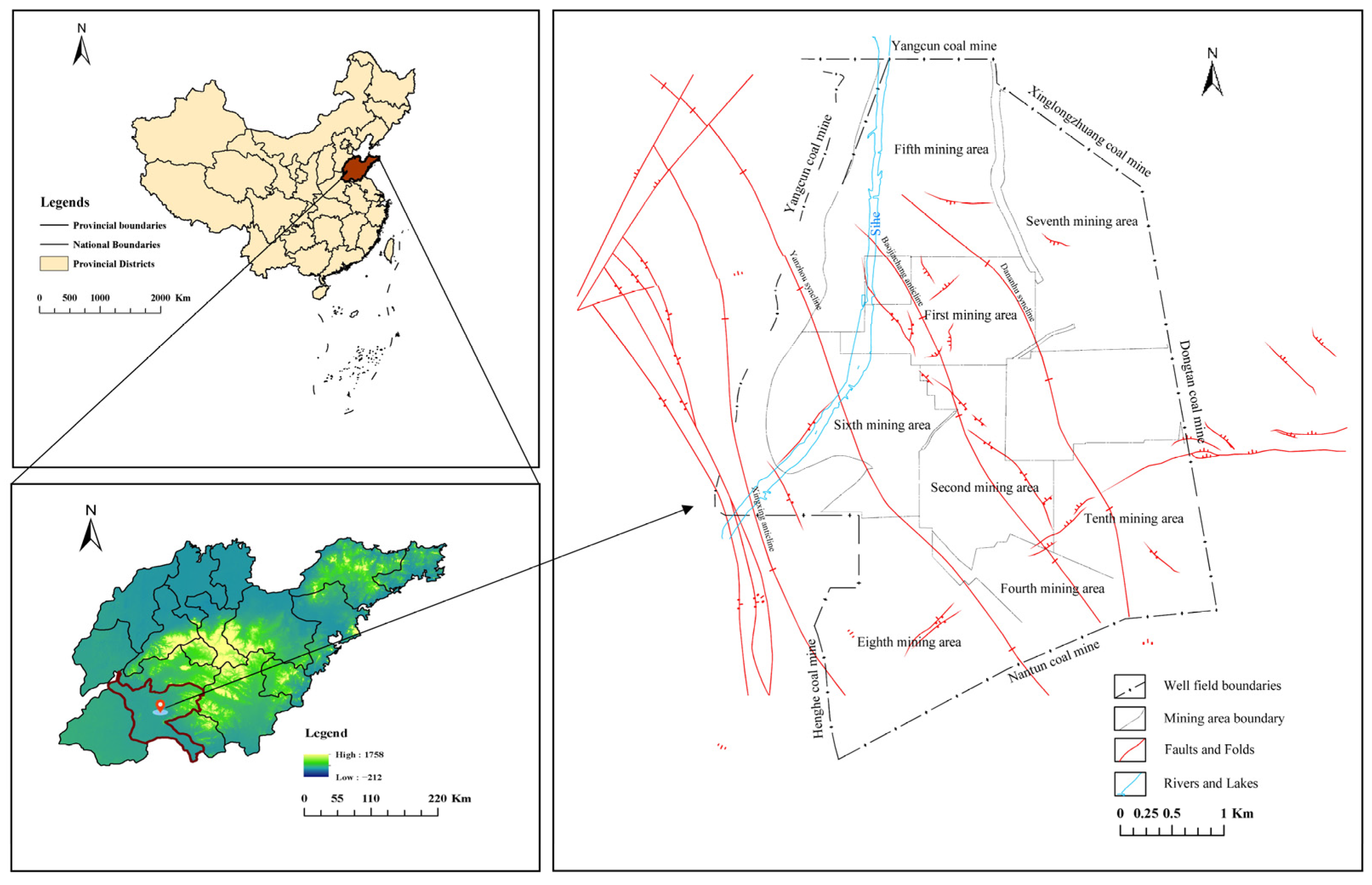
Figure 2.
Thematic map of indicators for water yield assessment: (a) Aquifer thickness; (b) Radius of influence; (c) Normalized drawdown; (d) Permeability coefficient; (e) Core recovery percentage; (f) Proportion of clay thickness to lower group thickness.

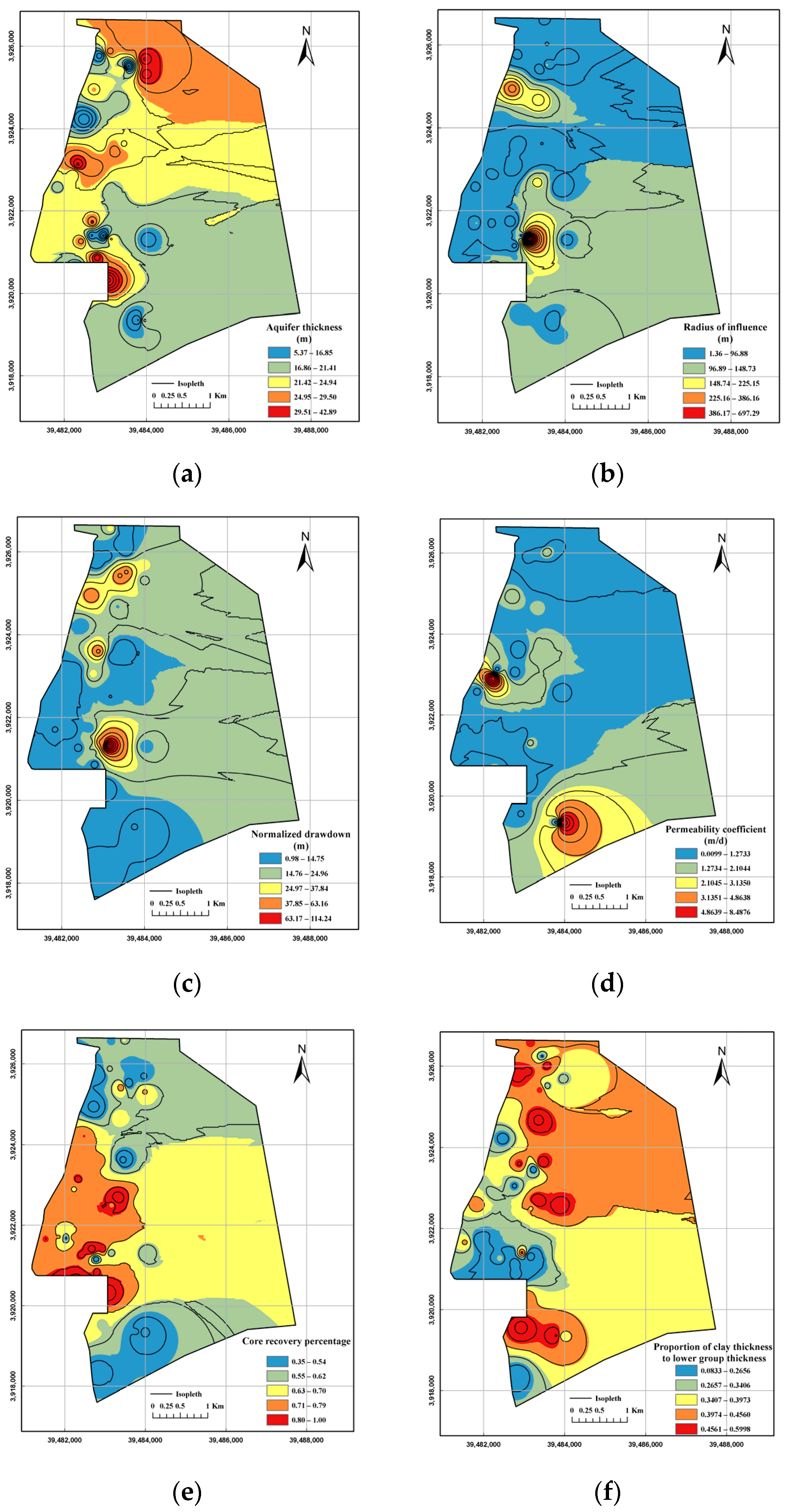
Figure 3.
Schematic diagram of CNN structure.

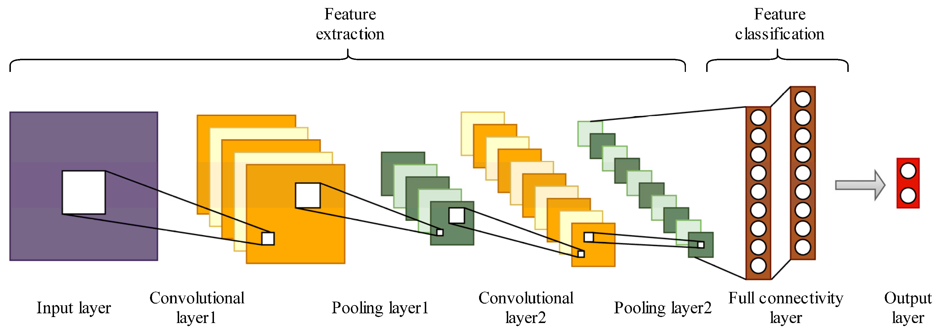
Figure 4.
Flowchart of CNN-SVM algorithm.

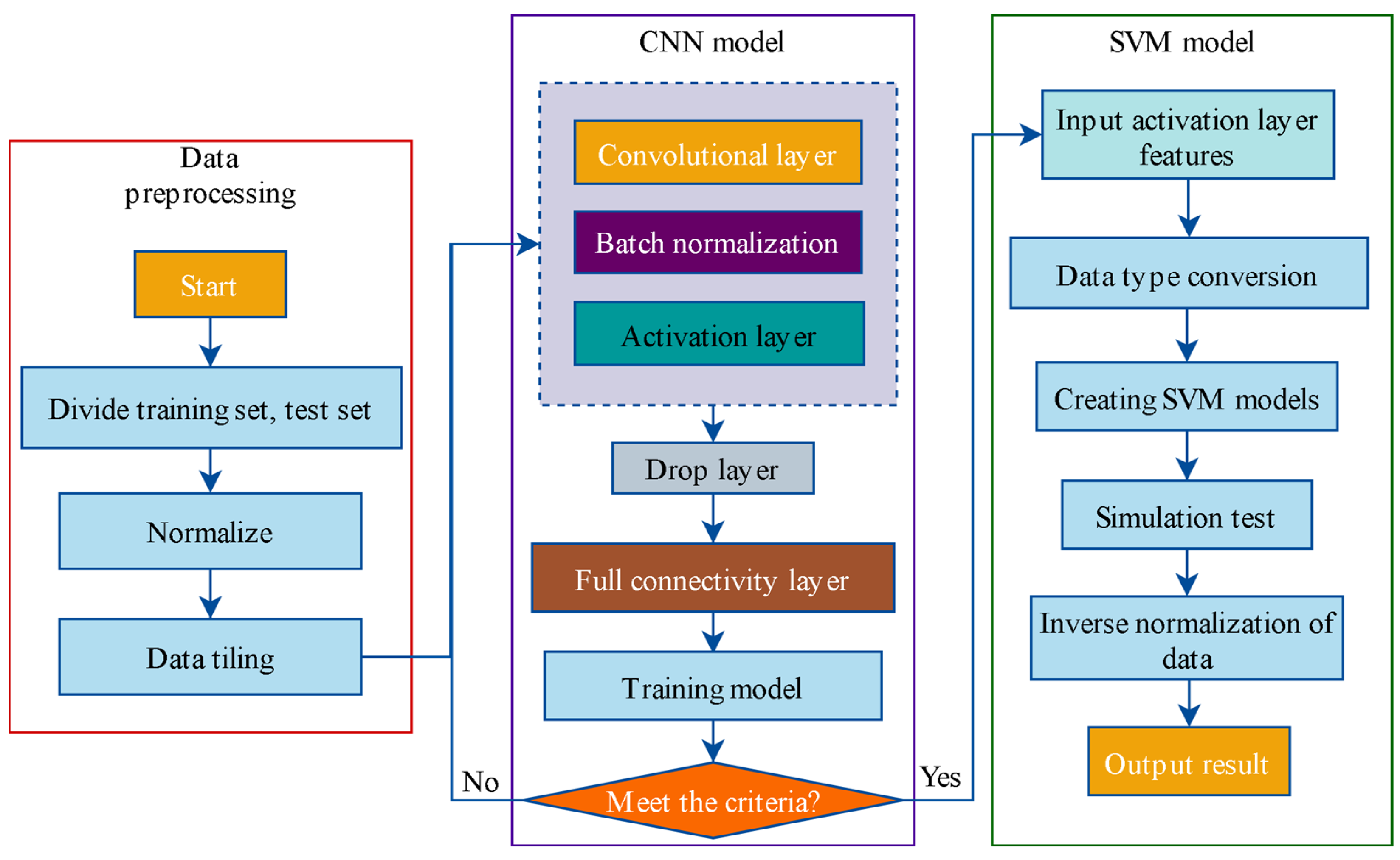
Figure 5.
Flowchart of WOA-CNN algorithm.

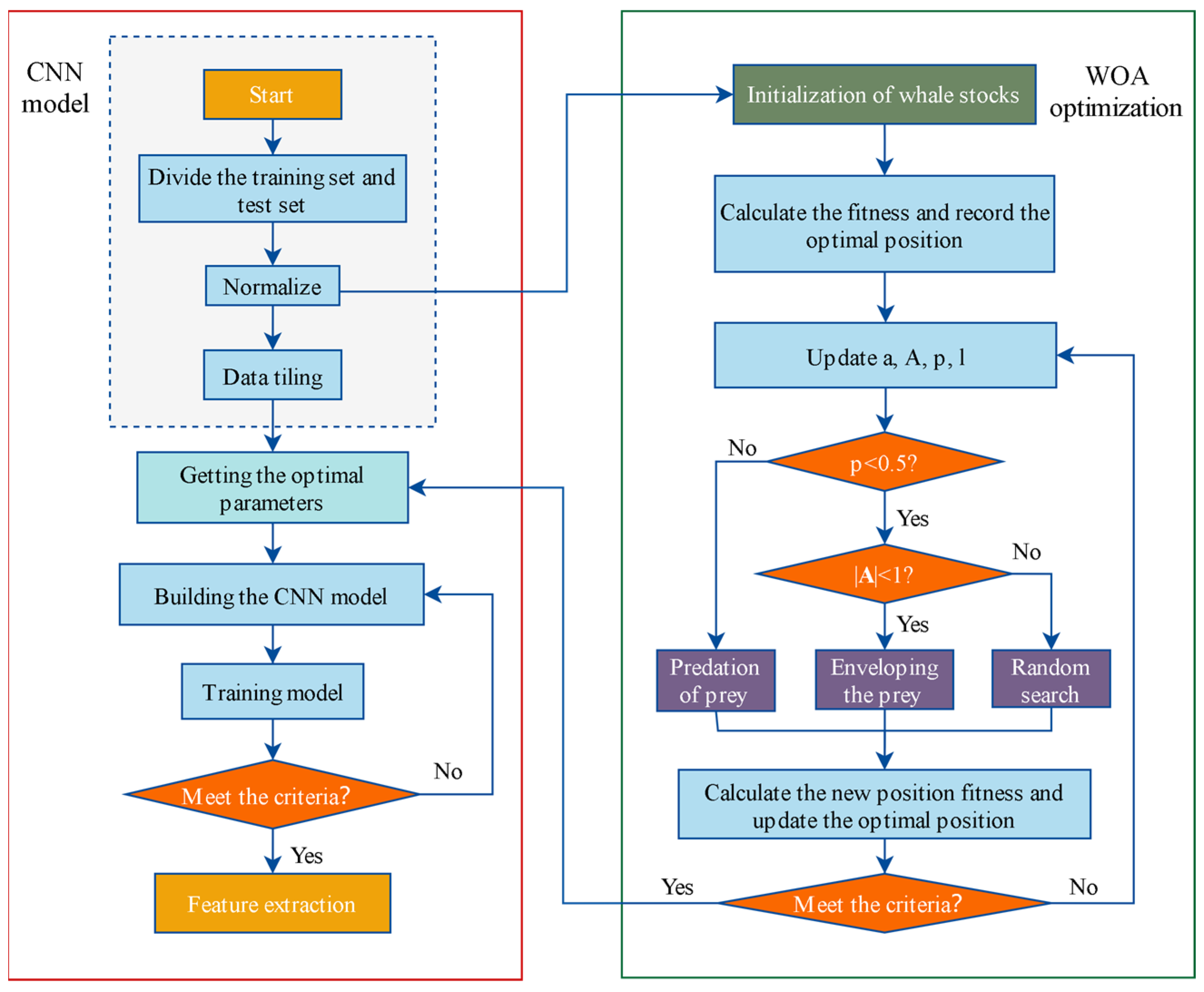
Figure 6.
Sample prediction process and results: (a) Loss curves; (b) Predicted versus true values of training samples; (c) Test sample predicted versus true values.

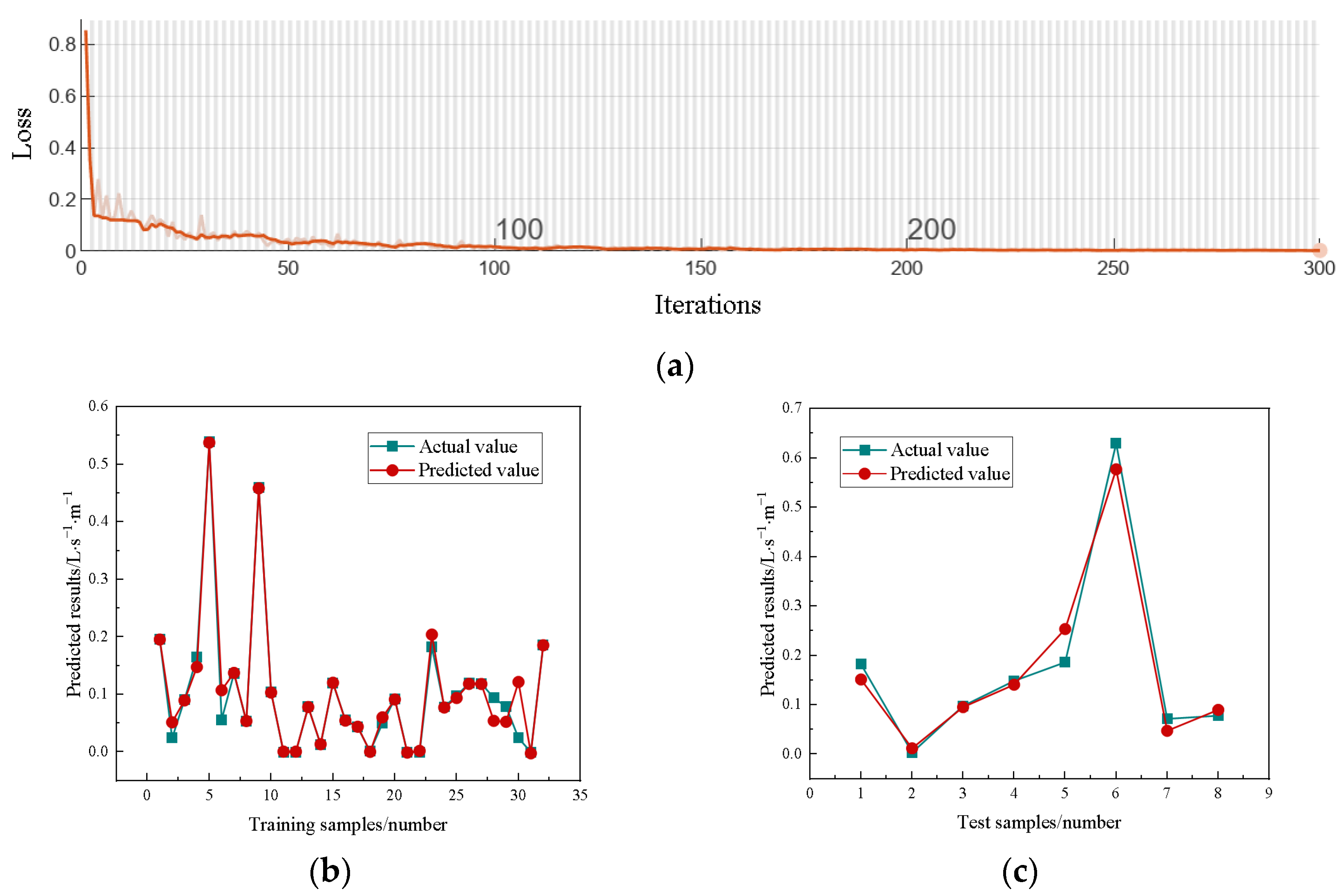
Figure 7.
Comparison of predicted and real values: (a) SVM; (b) CNN; (c) WOA-SVM; (d) WOA-CNN; (e) CNN-SVM; (f) WOA-CNN-SVM.

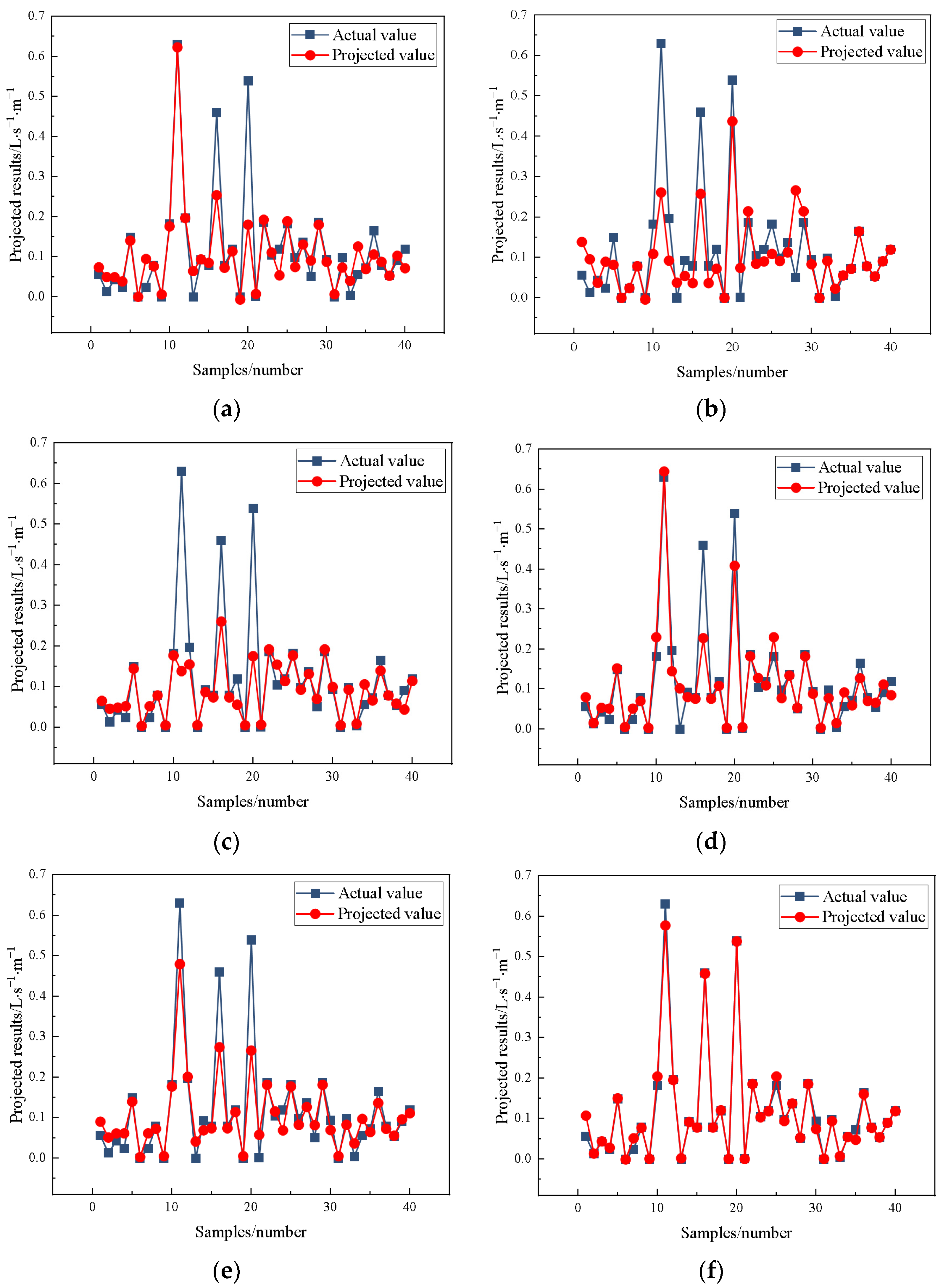
Figure 8.
Comparison of predictive performance of different models: (a) Optimized vs. unoptimized models; (b) Optimization model vs. other models.

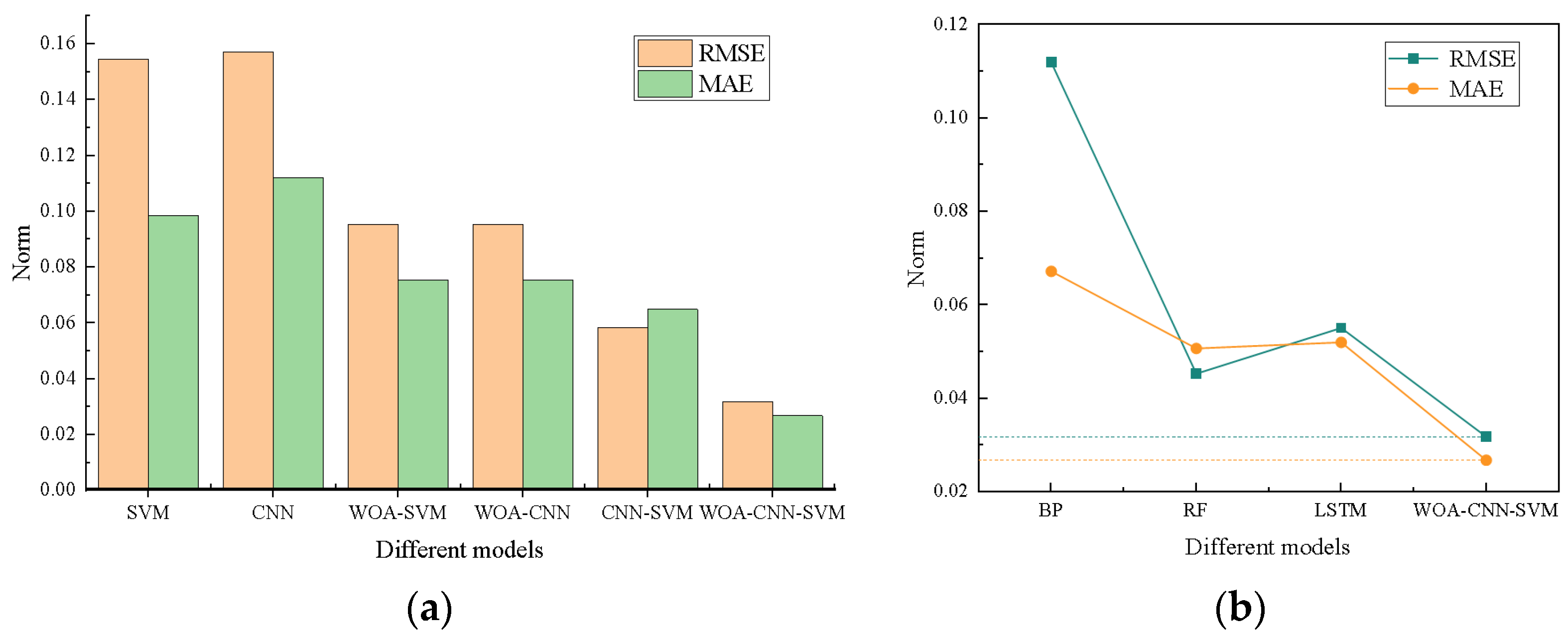
Figure 9.
Thematic map of water yield zoning in the study area: (a) Divided according to regulations; (b) Natural breakpoint method partitioning; (c) 3D surface map.

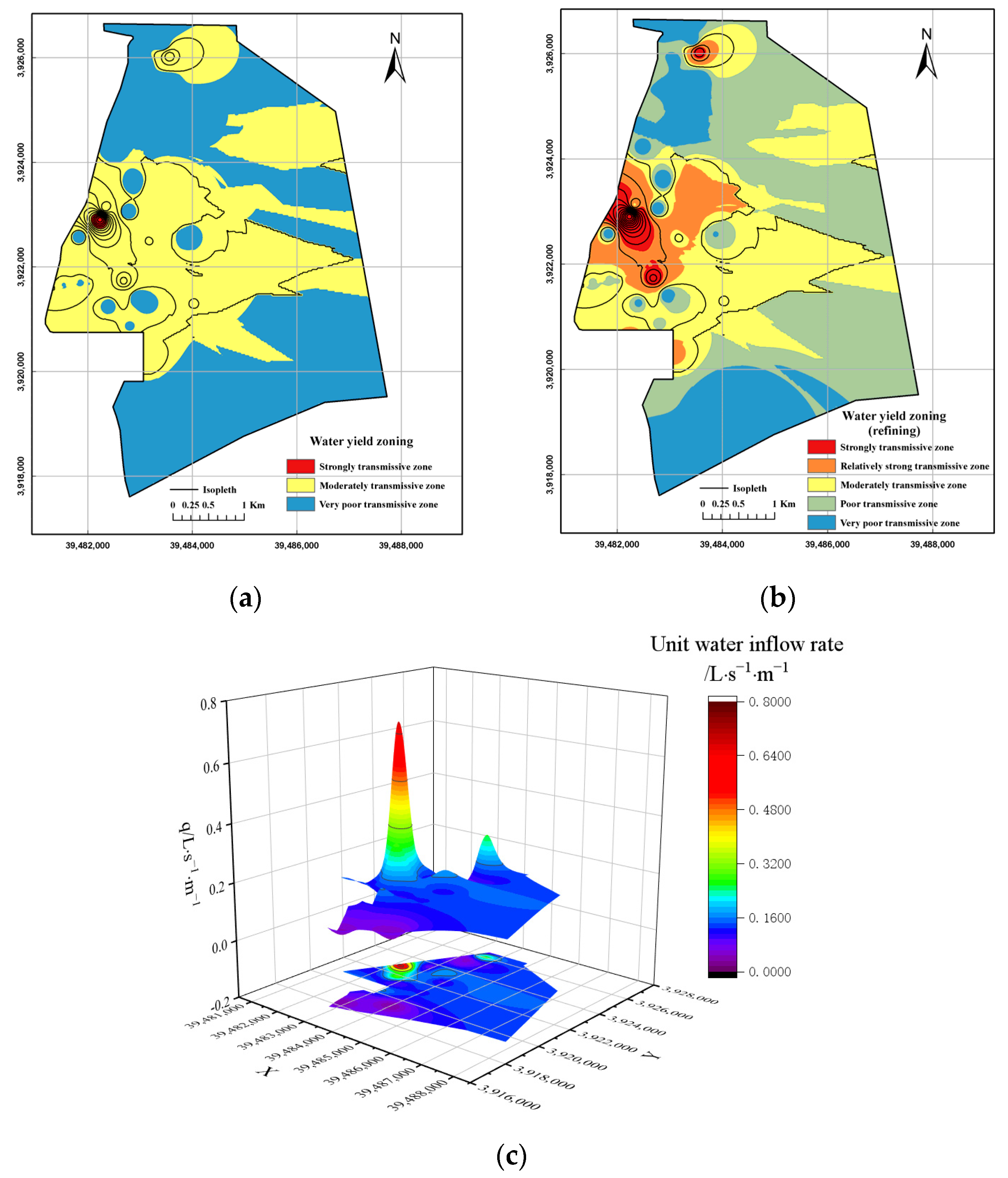
Table 1.
Water Yield Index Value.

Drill Hole Number	Dominant Factors						Unit Water Inflow Rate/ L·s⁻¹·m⁻¹
Drill Hole Number	X₁/m	X₂/m	X₃/m	X₄/m·d⁻¹	X₅	X₆	Unit Water Inflow Rate/ L·s⁻¹·m⁻¹
1	29.00	23.61	3.63	0.42	0.62	0.43	0.05
2	23.61	5.00	51.78	0.03	0.76	0.48	0.00
3	13.35	66.47	11.52	0.90	0.55	0.39	0.12
4	35.10	93.16	6.32	0.50	0.82	0.12	0.09
5	22.80	10.12	51.98	0.00	0.74	0.49	0.00
6	23.10	79.04	10.00	0.75	0.80	0.41	0.10
7	19.35	82.03	10.00	0.76	0.61	0.60	0.08
8	11.70	75.84	15.26	0.53	1.00	0.17	0.15
9	23.75	39.01	1.68	2.02	0.36	0.55	0.19
10	35.10	61.12	17.58	0.49	0.71	0.38	0.09
11	24.35	701.35	114.77	1.90	0.54	0.10	0.08
12	21.40	184.69	10.00	2.02	1.00	0.55	0.19
13	28.34	68.12	7.09	0.88	0.62	0.50	0.06
14	43.10	153.01	1.04	0.39	1.00	0.46	0.20
15	22.80	98.49	10.36	0.90	0.71	0.20	0.09
16	28.94	6.49	27.27	0.39	0.70	0.23	0.00
17	23.80	18.94	2.66	0.63	0.73	0.26	0.16
18	23.80	49.44	10.00	0.48	0.65	0.51	0.07
19	5.30	99.88	51.78	0.04	0.42	0.29	0.00
20	18.11	126.40	9.80	1.63	0.78	0.39	0.10
21	21.45	116.86	0.95	8.51	0.35	0.35	0.00
22	19.26	21.16	17.40	0.56	0.41	0.08	0.12
23	10.35	25.94	1.40	0.76	0.41	0.51	0.08
24	29.00	64.97	5.02	1.78	0.59	0.19	0.18
25	21.45	28.58	0.95	8.51	0.69	0.29	0.63
26	20.06	85.13	7.29	0.58	0.78	0.45	0.02
27	8.85	45.19	11.16	0.51	0.52	0.57	0.05
28	23.11	75.06	8.03	0.75	0.49	0.18	0.10
29	28.71	37.29	1.78	2.14	0.50	0.52	0.46
30	11.22	137.15	10.00	1.78	1.00	0.17	0.18
31	30.45	1.15	10.00	1.15	0.74	0.31	0.54
32	36.41	58.63	5.52	0.53	0.82	0.36	0.14
33	5.30	70.97	51.78	0.04	0.87	0.49	0.00
34	27.40	66.47	27.27	0.06	0.53	0.47	0.00
35	25.15	297.87	46.87	1.90	0.35	0.36	0.08
36	36.41	96.61	26.72	0.54	0.49	0.29	0.12
37	20.42	118.71	6.05	1.72	0.46	0.19	0.02
38	29.00	75.03	3.63	0.42	0.57	0.23	0.01
39	20.05	223.85	14.40	1.42	0.65	0.59	0.04
40	28.23	40.13	7.04	0.312	0.82	0.28	0.06

Table 2.
Unit water inflow rate prediction results.

Drill Hole Number	Dominant Factors						Projected Results /L·s⁻¹·m⁻¹
Drill Hole Number	X₁/m	X₂/m	X₃/m	X₄/m·d⁻¹	X₅	X₆	Projected Results /L·s⁻¹·m⁻¹
41	7.83	5.21	51.78	0.04	0.76	0.26	0.00
42	8.36	158.21	28.68	0.42	0.47	0.39	0.00
43	36.41	96.61	26.72	0.54	0.49	0.29	0.12
44	24.05	233.81	46.87	0.40	0.63	0.26	0.02
45	28.23	40.13	7.04	0.32	0.82	0.28	0.06
46	12.69	33.64	29.62	0.12	0.07	0.36	0.05
47	7.12	23.17	24.55	0.45	0.01	0.12	0.05
48	22.03	12.57	17.35	0.13	0.01	0.26	0.02
49	17.25	45.12	69.22	0.44	0.01	0.07	0.14
50	15.44	18.69	11.62	0.26	0.07	0.46	0.05

Disclaimer/Publisher’s Note: The statements, opinions and data contained in all publications are solely those of the individual author(s) and contributor(s) and not of MDPI and/or the editor(s). MDPI and/or the editor(s) disclaim responsibility for any injury to people or property resulting from any ideas, methods, instructions or products referred to in the content.

© 2024 by the authors. Licensee MDPI, Basel, Switzerland. This article is an open access article distributed under the terms and conditions of the Creative Commons Attribution (CC BY) license (https://creativecommons.org/licenses/by/4.0/).

[ad_2]