Assessing capacitance soil moisture sensor probes’ ability to sense nitrogen, phosphorus, and potassium using volumetric ion content

By inergency On Feb 8, 2024

[ad_1]

1 Introduction

Agricultural, urban, and industrial water resource management continue to play a significant role in eutrophication within freshwater systems, driven by factors such as population growth and intensification (Lu and Tian, 2017; Wurtsbaugh et al., 2019). It’s been shown that the management of irrigation and fertigation has major impacts on the nutrient leachate and runoff coming from agricultural production (Pérez-Martín and Benedito-Castillo, 2023). One approach to optimize agricultural production and minimize the environmental impacts involves high-quality diagnostic soil, plant, and water testing (Mylavarapu, 2010). However, a fraction (25%) of surveyed farmers in the USA and Australia conduct soil tests for monitoring nutrients (Lobry De Bruyn and Andrews, 2016). Due to these factors, the need for real-time soil nutrient monitoring is steadily increasing within agricultural water management. Such monitoring can contribute to the optimization of farmers’ fertilizer application rates and assist in implementing effective nutrient management practices (Burton et al., 2020), thus reducing agriculture’s impacts on water quality.

To promote wider adoption of nutrient monitoring techniques, several advancements in precision agriculture have emerged to assess plant and soil nutrient content at the field level. Optical sensors, satellite-based remote sensing technologies, and drone-based approaches have been gaining ground (Hunt and Daughtry, 2018; Inoue, 2020; Sishodia et al., 2020). While these technologies are nondestructive, they are expensive and require skills and knowledge in data processing before the farmers can effectively use the collected data for decision-making. Currently, the use of remote sensing technology is mainly limited to researchers (Weber and McCann, 2015; Bramley and Ouzman, 2019). An alternative approach for continuous field-level data acquisition involves in-ground sensors. Capacitance soil moisture sensors (SMS) for instance, provide real-time readings of soil water (SM), volumetric ion content (VIC) or electrical conductivity (EC), and soil temperature (T). These sensors provide two outputs from dimensionless frequencies that within conjunction with one another, give readings of volumetric water content and VIC when separated by proprietary data model processes. (TriSCAN ® Agronomic User Manual Version 1.2a, 2003, Adelaide, Australia). The VIC data derived from SMS represents the dielectric constant, which is influenced by the presence of salts from fertilizers and irrigation water. If nutrient salts from fertilizers significantly impact the soil osmotic potential, the sensor can detect them (Or and Wraith, 2002). The use of SMS for optimal irrigation scheduling has been adopted more by farmers than any other technology-based irrigation scheduling technique in the USA (Taghvaeian et al., 2020). If this most-adopted approach could also be utilized for nutrient management, the rate of adoption could be greatly increased. Based on the VIC-EC measuring capabilities of SMS’s and soil moisture probes (SMP), it’s hypothesized that a similar approach could potentially be employed for nutrient monitoring and management, in addition to irrigation scheduling using SMS VIC data, if relationships between nutrient movement across the soil profile and VIC readings are established. If this connection is successfully established, decision support systems could utilize this already commercially-available and adopted technology to quickly diffuse fertigation management strategies, decreasing agriculture’s contributions to eutrophication. It is known that decision support systems already utilize sensor outputs for the management of irrigation and fertigation practices to reduce environmental impacts (Zhai et al., 2020). But first, before implementation into systems as a nutrient-sustainable management strategy, it must be investigated which nutrients the technology could potentially be detecting.

It’s hypothesize that in-ground SMS could be sensitive to nutrient movement in the soil. This hypothesis arises from three known principles. First, the nutrients’ influence on EC (Omonode and Vyn, 2006; Mirzakhaninafchi et al., 2017; Darmawan et al., 2023). Second, the established correlation between soil cations/anions and EC (Friedman, 2005), and third, the sensors’ capacity to detect soil VIC. Notably, fertilizers containing Nitrogen (N), Phosphorous (P), and Potassium (K) are known to increase EC (Bhatt et al., 2019). The SMS’s VIC measurements have been found to be directly correlated to soil EC, with variation across soil types (Biswas et al., 2007). This correlation indicates the potential of SMS to detect the presence of N, P, and K in the soil due to fertilizer applications, inferred from VIC data. To the best of our knowledge, no published studies have examined the capability of these capacitance SMS to detect N, P, and K movements individually. In this study, laboratory-based experiments were conducted to assess the changes caused in the VIC time series from SMS due to the presence of N, P, and K in a pure sand media. While the SMS’s VIC sensing capabilities make direct nutrient detection unlikely, the ability to indirectly indicate high nutrient content in the soil holds value for those utilizing the sensors for management or those creating decision support systems in precision agriculture. Given that these SMS are readily available on the market and are being used by farmers in the USA, they could represent a feasible and rapid solution for implementing efficient in-field nutrient management plans. However, there is a need for them to be investigated to fully understand which nutrients are in fact being detected by the sensors. By harnessing real-time data, these systems could both maintain optimal agricultural water and nutrient management while minimizing environmental impacts from crop production.

2 Materials and methods

2.1 Experiment location, design, and treatments

The three N, P, and K experiments were conducted individually at the University of Florida’s Indian River Research and Education Center in Fort Pierce, FL, USA (27°25’33.9″N 80°24’29.4″ W). The laboratory was kept at a constant temperature of around 21°C. While constant temperature cannot be expected in field settings, this study was designed to minimize any variation in the time series created from temperature variances, so the SMS signals were mostly influenced by each nutrient. Each experiment followed similar protocols and had a randomized complete block design where the SMSs data collection over a 24-hour time was considered the replication or block (Figure 1). Specifically, the N and K experiments encompassed three distinct rates and were replicated three times, while the P experiment tested two different rates of P and had five replications. Sequentially, the P experiment was conducted initially, followed by the N and K experiments. After concluding the P experiment, it was determined that the N and K experiments would benefit from more rates and fewer repetitions. This was determined due to literature pointing stronger to impacts of N and K on soil EC (Carneiro et al., 2017; Guo et al., 2021) while it pointed to smaller impacts of P on soil EC (Ding et al., 2020). As previous studies showed weaker P impact on soil EC but still impacting, it was determined to be beneficial to investigate 2 application rates of P which were significantly different from each other with higher numbers of repetitions to determine if P would be detectable through the SMP. However, as previous studies successfully registered strong EC signals from N and K in soils, it was determined to be beneficial to further investigate how sensitive the SMSs could be to various application rates of N and K beyond simple detection. Despite the differences in number of repetitions and applications between the three separate experiments, each experiment had a randomized complete block design where the 24-hour time was considered the replication or block. A summary of the treatments and nutrient rates used in this study is outlined in Table 1.

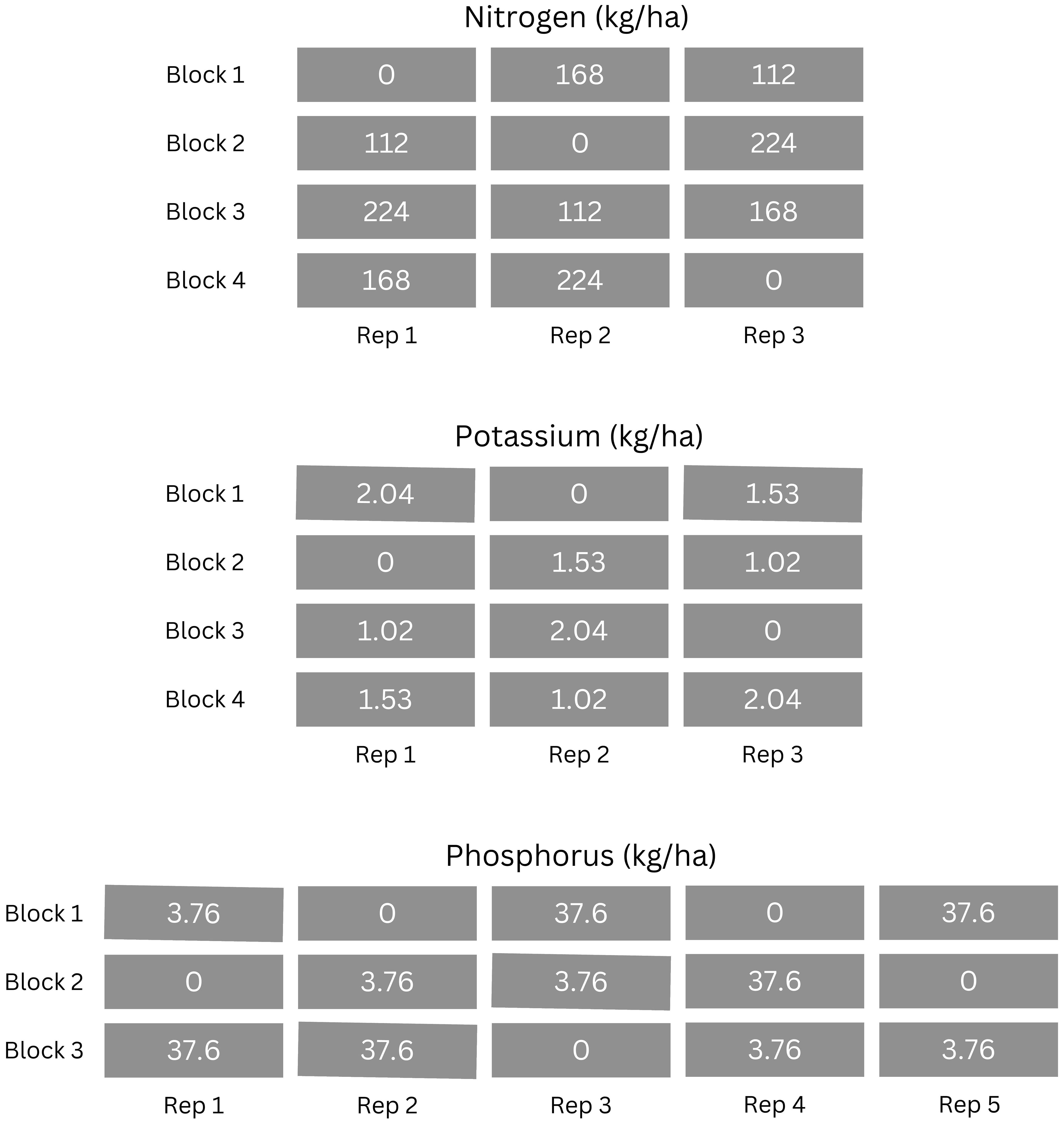
Figure 1 Diagram of the randomized complete block design for N, P and K experiments.

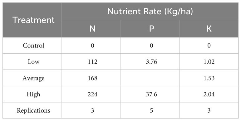
Table 1 N, P, and K rates per treatment.

The N source used was powdered urea (42-0-0), and the N rate treatments were application rates selected based on local N fertilizer recommendations for sweetcorn (Hochmuth and Hanlon, 1995). The low rate indicates split application at the six-leaf stage of the crop, the average rate is the preplant application rate, and the high rate represents the total accumulated N suggested for one crop season. For P a 1000 ppm orthophosphate standard solution was purchased from Fisher Scientific. This solution was selected as inorganic P is a bioavailable source of P (Thien and Myers, 1992) often found in fertilizers (Cade-Menun et al., 2017). P rates were determined based on soil P concentration of a local sweetcorn farm in South Florida, USA, where the high rate represented average P soil levels, and the low rate was one-tenth of this level. The K source was KCl 3M solution from Fisher Scientific, with treatments selected based on groundwater salinity concentrations. According to Her and Vassilaros (2022), the maximum groundwater salinity concentration reported was 9.12 dS/m along the South Florida coastal areas. Thus, in this study, this measurement was used as a baseline to convert K levels ranging from 5-10 dS/m reflecting groundwater levels (Her and Vassilaros, 2022) to the kg/ha measurements of 1.02, 1.53, 2.04 kg/ha treatments. Each nutrient source was mixed with 500 ml reverse osmosis water, and to ensure consistency in metrics, units were transformed to nutrient rates per hectare of land.

2.2 Soil moisture probe and calibration

A TriSCAN Sentek drill and drop (SMP) soil moisture probe (Sentek Drill and Drop SDI-12 Series III, 2015) was utilized for this experiment. The SMP is equipped with 6 individual SMSs distributed equally down the probe. Across the SMP, sensors are located at specific depths: 5 cm (sensor 1), 15 cm (sensor 2), 25 cm (sensor 3), 35 cm (sensor 4), 45 cm (sensor 5), and 55 cm (sensor 6) from the surface. Each SMS provides readings of volumetric soil water content, soil temperature, and VIC at 15-minute intervals. The sensors generate two frequencies. The first frequency is converted through a normalization Equation 1 (Schelter et al., 2006).

and calibrated to volumetric soil water content. The second frequency is proportional to soil water content and the presence of free ions in the soil pore water. Proprietary data modeling integrates changes in both signals, yielding nominal VIC. These VIC readings can also be correlated with EC (Sentek TriSCAN ® Agronomic User Manual Version 1.2a, 2003, Adelaide, Australia). When the SMP is inserted into soil, each sensor within the SMP begins transmitting the soil water content, soil temperature, and VIC data in real-time every 15 minutes, generating a time series that begins from the moment of installation. This data can be observed by the user on commercial displays developed by data providers for service. Multiple data providers service the SMP used in this study. To ensure uniform measurements across all sensors, the SMPs were calibrated according to Sentek Technologies’ soil moisture sensors calibration manual (Calibration Manual for Sentek Soil Moisture Sensors Version 2.0, 2011). For each soil core, a single SMP was installed as shown in Figure 2. Data from the SMPs were retrieved via two data providers currently being used within the state of Florida: BMP Logic (https://www.bmplogic.net/) and Pessl Instruments (http://metosusa.com/). The subsequent data analysis was performed on the raw data extracted from each platform.

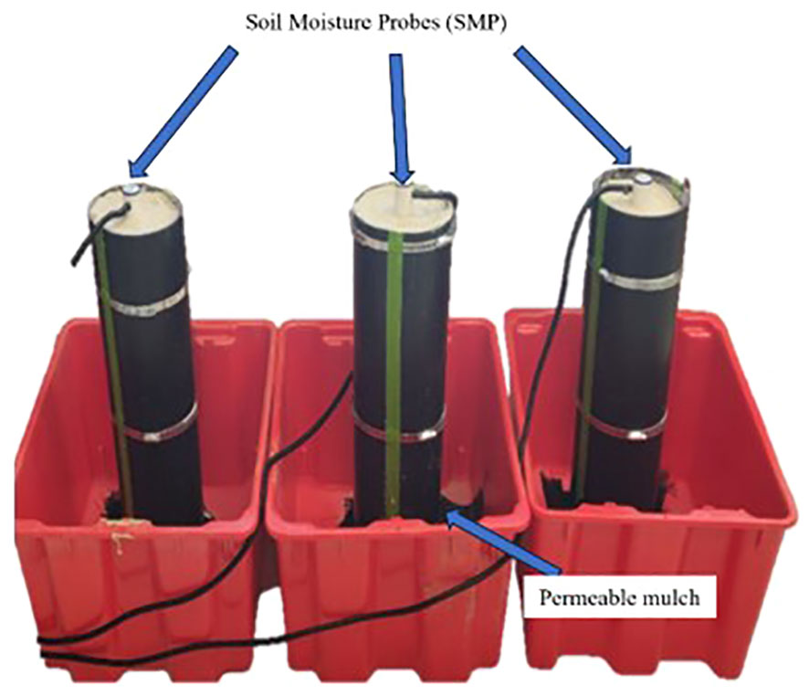
Figure 2 Laboratory experimental setup pre-nutrient application.

2.3 Experimental protocol

Soil cores were composed of 60 cm tall riser-pipe cylinders with a 16 cm diameter. Each cylinder was cut through the middle lengthwise, and fitted together with hose clamps, with the aim of replication sampling (Figure 3). To prevent soil movement with leachate, the lower portion of the pipes were sealed using a water-permeable fabric mulch. The fabric mulch ground cover utilized in this study was manufactured by Lumite, Inc (http://www.lumiteinc.com/products/groundcover) and is comprised of a blend of woven fabrics and UV polypropylene that allows passage of water and nutrients at a rate of 720 L min/m2.

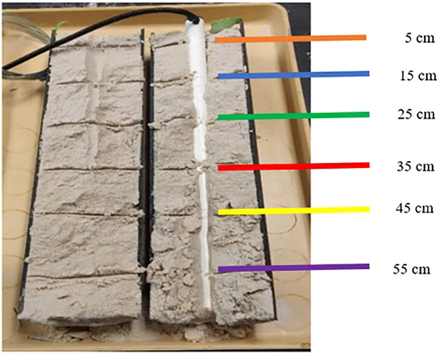
Figure 3 Sand core and extraction of soil samples for laboratory analysis based on the sensor depth. Horizontal colored lines represent the location of each soil moisture sensors across the core.

The cores were filled with 15 kg of silica sand and evenly trapped along the sides in a uniform manner to prevent air gaps. To avoid variance in compaction, cores were only proceeded to be used if greater than 2.5 yet less than 5 cm of space was present at the top of the core. As each core held the same mass of sand and was equal in volume, anything outside of these parameters was determined to have a variance in compaction and was not used in the experiment. SMPs were installed in the center of each core following the manufacturer’s installation protocols (Sentek Drill and Drop SDI-12 Series III, 2015). Following SMP installation, the cores remained undisturbed for 1.5 hours to allow for temperature adjustment and soil settling. Subsequently, the 500ml solution containing either N, P, or K was applied. The solution was evenly poured onto the core’s surface using a custom-made strainer, ensuring uniform distribution across the top surface. After the solution had thoroughly passed through the strainer, the core remained undisturbed for 24 hours.

At the end of the 24-hour period, the SMPs were carefully positioned horizontally to prevent further seepage. The core was then divided into six distinct 10 cm sections (Figure 3), corresponding to the descending depths of sensors within the SMP. These soil sections were compositely, air-dried for P and K or stored in the refrigerator for N, before being sent for analysis. N and K soil samples were sent to Water’s Agricultural Laboratory (Camilla, GA) for extraction and analysis while P soil samples were sent to UF IFAS Everglades Research and Education Center’s soil lab for Mehlich III extraction and analysis.

2.4 Data analysis

The time series obtained per treatment were evaluated by assessing three VIC points within the time series and their comparison by ANOVA. These points attained were identified as the maximum point (MP), inflection point (IP), and the convergence point (CV). The MP was evaluated in two ways: the MP value (MPv) and its time of occurrence (MPt), which together represent the highest VIC reading given by the SMS within the SMP at its given depth. The inflection point was also evaluated in two ways: the IP value (IPv) and its time of occurrence (IPt), which together represent the slope of drainage after the nutrient solution has passed down to deeper soil layers, or the soil is under its water-available field capacity conditions. The CV was only evaluated in value as it is the final normalized value taken after 24 hours, making its time of occurrence equal in each repetition. The CV represents the ‘settling point’ of the solution. A visual representation of these points is displayed in Figure 4. Graphs were obtained from each repetition of each treatment; Figure 4 is a sample of the first repetition in the K experiment presented here as a visual guide.

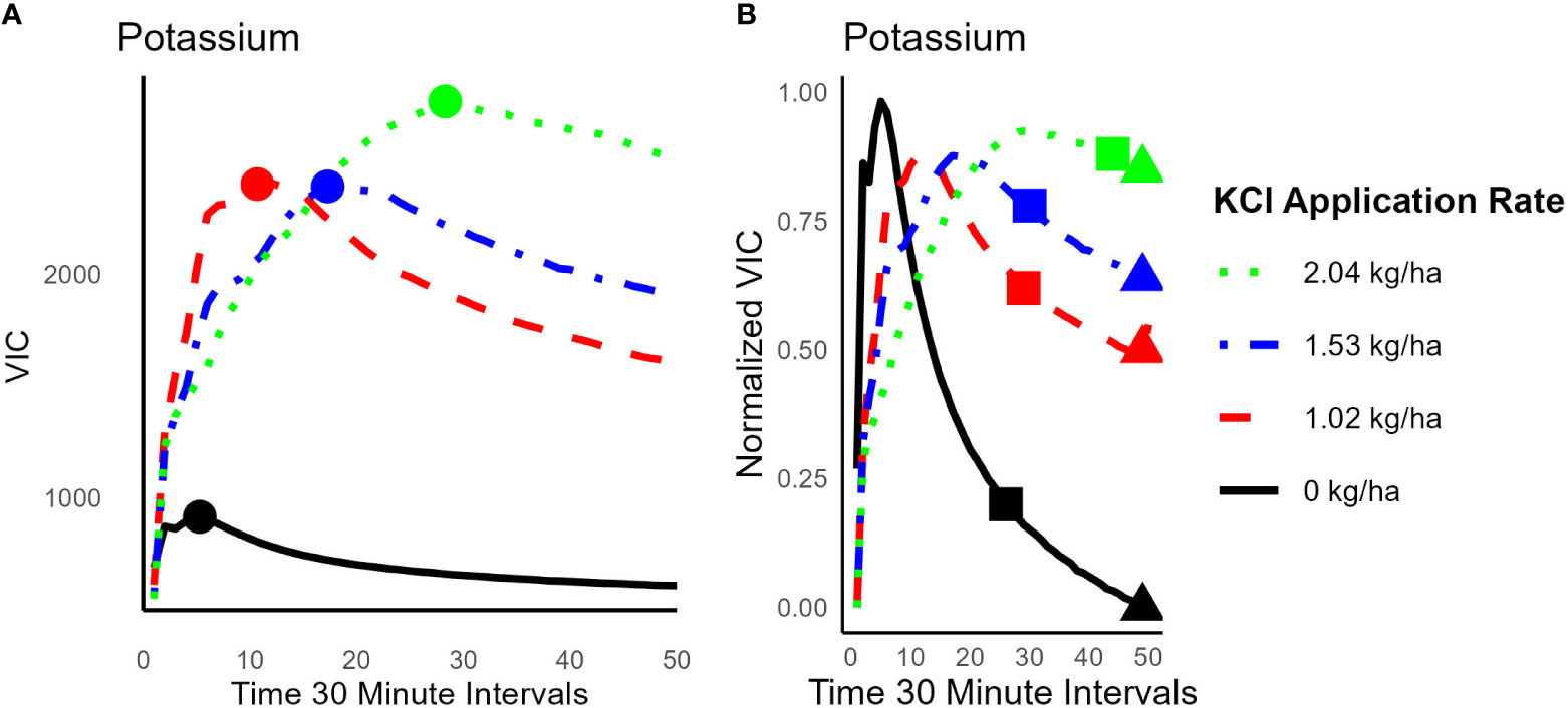
Figure 4 Identification of signal dispersions in the time series from raw data (A) and normalized data (B) from the potassium trial at 5 cm depth. Circles represent the maximum points per treatment (MP), squares represent inflection points per treatment (IP), and triangles represent the convergence points per treatment (CV).

As the purpose of this research is to evaluate these currently used SMP’s ability to detect nutrients in the soil, it was important that the elements of the VIC curve analyzed were elements that reflect the current time series management for irrigation scheduling by farmers. the University of Florida Electronic Data Information Source (EDIS) offers guidelines to interpret time series elements and values to assist growers in irrigation management (Zotarelli et al., 2019). The MP value in this study is equivalent to what a grower would identify as the irrigation event peak during an irrigation event. IP represents the major change in the time series slope (Phlips et al., 2021), which is similar to the practical method used by growers to identify soil field capacity, or the ‘slope of drainage’. CV represents the final value in the time series where there is no more downward movement of nutrients. This is the only value that can be directly compared to the laboratory analysis as it is static.

Following the identification of the MPs, the raw time-series data $Y = ({y_{1}, y_{2}, \dots, y_{n}})$ was normalized to a range of (0,1) for IP and CV identification. IPs were detected using the changepoint algorithm following the description from Killick and Eckley (2014), and adapted as follows in Equations 2–4:

Let $(y_{1 : n})$ represent the sequence of data points from the first $(y_{1})$ to the last observation in the time series $(y_{n}) .$ Under the null hypothesis $(H_{0})$ , it is assumed that no changepoint exists in the time series. Let $(L_{0})$ be the maximum log-likelihood under this hypothesis, which is defined as:

Here, $p (\cdot)$ represents the probability density function associated with the distribution of the data, and $\hat{θ} = [\hat{μ}, \hat{σ}]$ is the maximum likelihood estimate (MLE) of the mean and standard deviation that best fit the distribution of $Y$ .

Under the alternative hypothesis $(H_{a})$ , a changepoint at $(τ_{1})$ is assumed to exist. Let $L (τ_{1})$ be the maximum log-likelihood under this hypothesis, which is defined as:

\begin{array}{l} L (τ_{1}) = log p (y_{(1 : τ_{1})} | {\hat{θ}}_{1}) + log p (y_{(τ_{1} + 1 : n)} | {\hat{θ}}_{2}) & (3) \end{array}

The likelihood ratio test statistic $λ$ is constructed using $L_{0}$ and $L (τ_{1})$ , and is defined as:

\begin{array}{l} λ = 2 [max_{τ_{1}} L (τ_{1}) - L_{0}] & (4) \end{array}

Therefore, the test is performed by selecting a threshold (c) such that the null hypothesis is rejected if $λ > c$ . If the null hypothesis is rejected the position $τ_{1}$ is estimated and considered as the detected changepoint

Following the identification of the MP, IP, and CV values, the one-way ANOVA followed by the post hoc Tukey test was performed to identify differences among the treatments. By utilizing ANOVA, MPs IPs and CVs could be compared across application rates, and immediately determine if the MPs IPs and CVs changed in a significant matter with the application of N, P, or K. Significant changes in MP IP or CV would indicate the SMPs’ sensitivity to the presence of the nutrient, while the absence of significance would indicate a lack of SMPs’ sensitivity to the presence of the nutrient. The two-way ANOVA followed by post hoc Tukey was performed on the laboratory analysis results for the N, P, and K using both treatment and SMS depth as variables to understand the individual variable impact and their interactions. The remaining of this study will use the following nomenclature for clarity in the results. ‘Experiments’ will refer to the entire set of measurements taken from either N, P, or K. ‘Applications’ will refer to the nutrient rates applied, including the control, low, average, and high application rates. ‘Repetition’ refers to how many times the applications were repeated. For example: The 1^st repetition of the low application in the N experiment would refer to the time series obtained from the first time the low nitrogen nutrient application was applied to a core.

3 Results and discussion

3.1 Maximum point

3.1.1 Value of maximum point

Among the three tested nutrients, only K has significant differences (Table 2). The analysis of MPv differences related to K was approached by comparing MPv across different treatments. When comparing MPv per depth and application rate, an increase in MPv was observed in direct correlation with each application rate except at 15 cm depth, where the highest K application yielded a lower MPv than the low and average applications (Figure 5). Results from the control treatment showed that the top five SMSs displayed similar MPv, ranging from 894-945 VIC units. However, the sixth SMS, situated at 55 cm depth, recorded a VIC measurement of 1079 units, which is higher than the readings of the top five sensors. This deviation might be attributed to a change in sensor sensitivity, due to increased soil water resulting from downward water movement within the soil core, In this context, higher water content leads to a higher VIC reading.

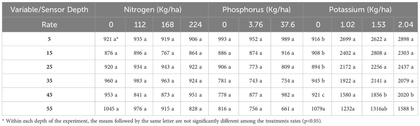
Table 2 ANOVA maximum point value means for N, P, and K treatments at each sensor depth (5-55 cm).

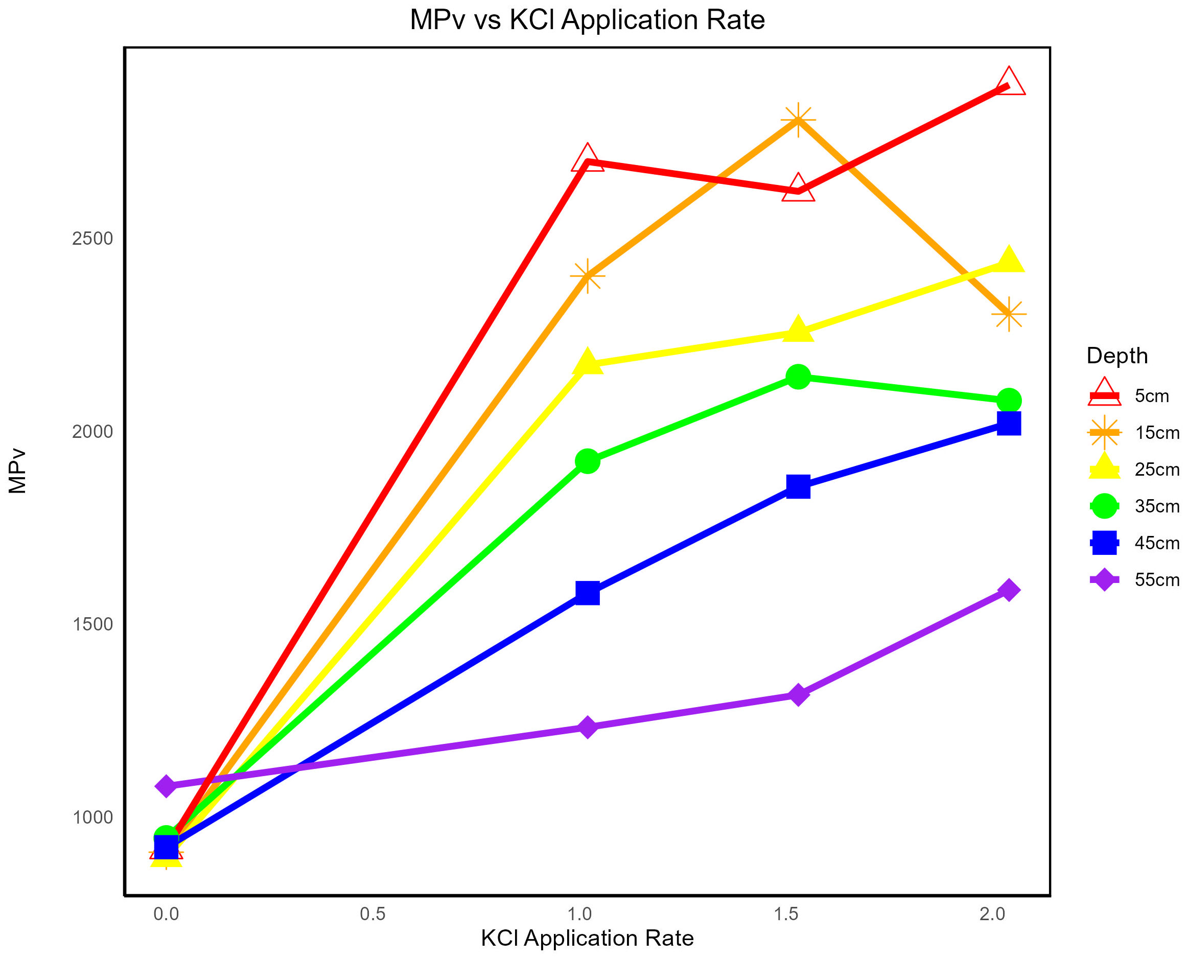
Figure 5 Maximum Point Values (MPv) averaged per repetition in relation to the K (KCl) rate (0, 1.02, 1.52, and 2.04 kg/ha) at each sensor depth (5-55 cm).

The mean values displayed in Table 2 confirm that each K application rate resulted in a higher MPv than the control, as indicated by the Tukey letter groupings. However, while treatments were different from the control, they did not differ from each other in the 5-35 cm depths. There is an increase in MPv in the average and high treatments compared to the low treatment at 45 cm, and increases in MPv across all applications at 55 cm. A steady increase in MPv at those depths is observed as the concentration of K increases. Differences in VIC at the lower depths could be attributed to soil water influence. Soil water has an influence and positive correlation on the electrical conductivity (EC) of soils (Mojid et al., 2007). In a study conducted by Brevik et al. (2006), to understand the effect of soil water content changes on soil EC, it was shown that the electrical conductivity was greatly influenced by soil water.

3.1.2 Time of maximum point occurrence

After evaluating the MPt, it was evident that, among the three tested nutrients, only K exhibited significant differences. When comparing MPt at each depth within individual application rates, an increase in MPt was observed in direct correlation with each increasing application rate. Figure 6 shows that each application rate at each depth showed an increase in MPt compared to the control application. While every application yielded higher MPt than the control, the greatest application of K did not always result in the greatest MPt reached. In Figure 6, at the 15 cm depth, the highest K application yielded a slightly lower MPt than the average application. Table 3 shows that the difference between these values are statistically similar. The 5, 25, and 35 cm depths display a steady increase in MPt consistent with the increase in K application applied.

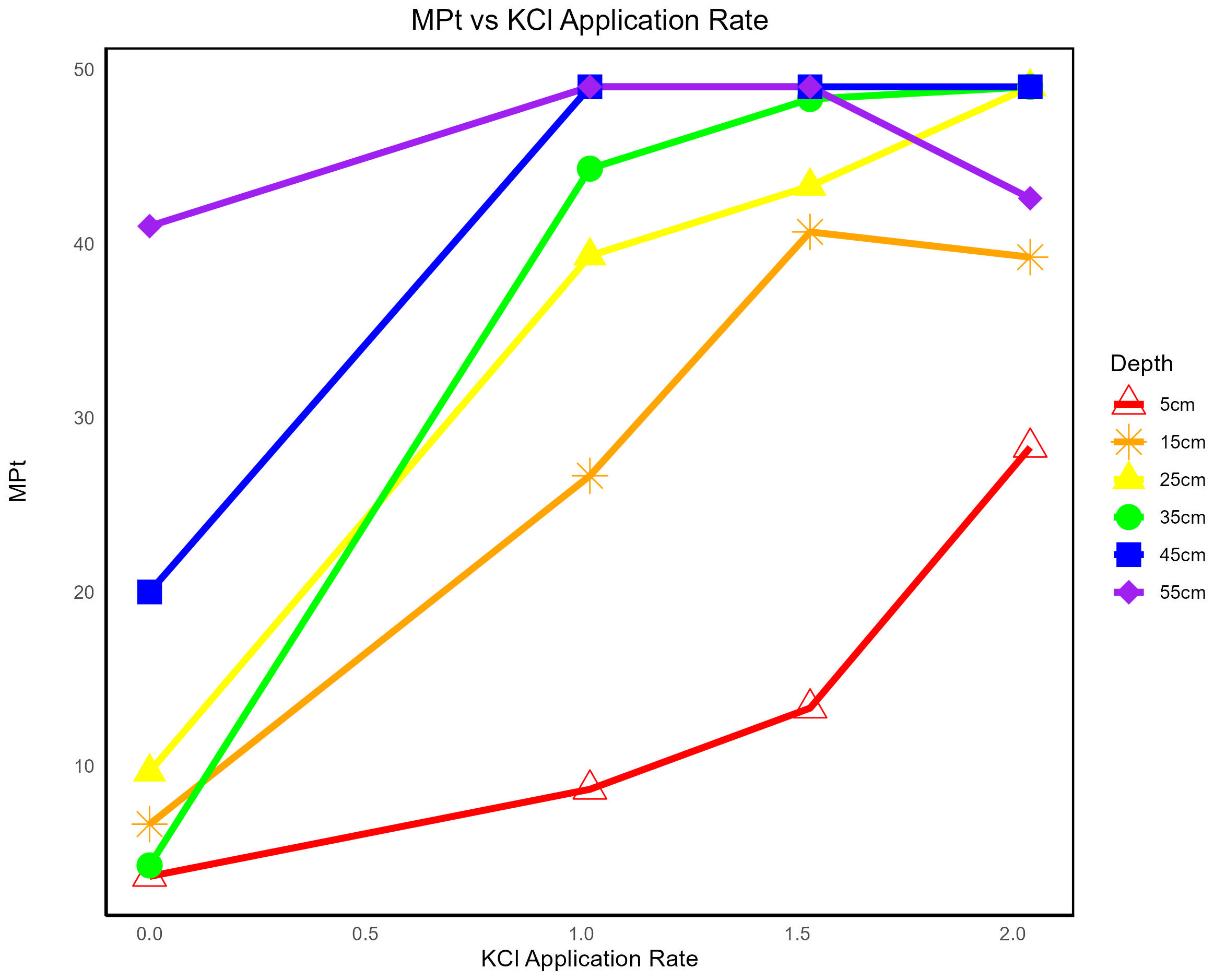
Figure 6 Maximum Point Time (MPt) averaged from each repetition in relation to the K (KCl) rate (0, 1.02, 1.52, and 2.04 kg/ha) at each sensor depth (5-55 cm).

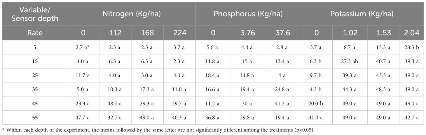
Table 3 ANOVA Maximum Point Time (MPt) means for N, P, and K treatments at each sensor depth (5-55 cm).

Table 3 shows that, from 15 cm though 45 cm depth, each K application yields a significantly higher MPt than the control. However, the increase in MPt at 5 cm depth is only significant for the high application rate if compared to the control. Furthermore, at 15 cm, the high and average application MPts are higher than the low application, showing the sensor ability to differentiate between application rates.

In this study, the sensor VIC changes are used as an indication of their sensitiveness to K presence and movement in the soil. As the VIC sensor readings are potentially impacted by soil water, it is possible that the presence of any nutrient increasing electrical conductivity has the potential to delay the MPt. This delay of the MPt could potentially be a method of K detection in soil media. These results are in accordance to the findings of Thompson et al. (2007), where it was shown that ,in a sand column experiment, the soil water content increases approximately 2-5% with 1 dS/m increase in the EC. Peddinti et al. (2020) used KCl to examine salinity effect on capacitance based sensor volumetric water content readings and observed similar results where the sensor’s sensitiveness to measuring volumetric water content is affected by soil solution salinity.

Table 4 shows that K generally remained in the top 30 cm of the soil core. These laboratory results were in agreement with the results obtained for MPt (Table 3), as the two depths with distinction between treatments are at 5 and 15 cm sensor depth, below the 30 cm mark. It was observed that there was a stronger difference in MPt at the 15 cm sensor than the 5 cm sensor, which could be attributed to K settling in that layer. The passage of K and the settling of residual K could have provided greater signal delay at 15 cm than at 5 cm. This phenomenon is observed for all K application rates. After 25 cm, each treatment’s MPt occurred at or very near the end of the 24 hours’ period. As there was only one water application for each repetition, this delay is likely the combined impact of water and K not reaching the depth until much later, as well as the possible overshadowing of the soil water signal over the lower application rates of K at those depths.

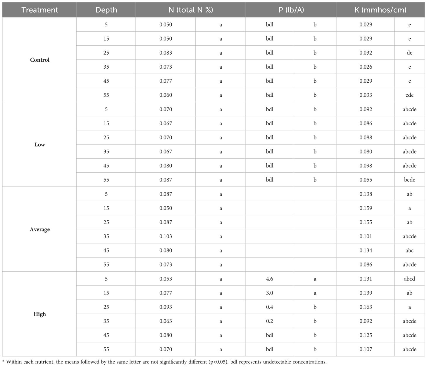
Table 4 ANOVA results from N, P, and K laboratory samples mean at various depths and rates.

Comparing the K results with those from N, there was not a MPt delay. This response could be attributed to the high mobility of N in water causing lesser accumulation of it at one depth, which therefore resulted in no impact on the MPt. NH₄⁺ is highly soluble in water and do not easily bind with the soil particles moving quickly through the core. According to Casey et al. (2002) the mobility and availability of N is increased with an increase in soil moisture. The low cation exchange capacity (CEC) of the pure sand media used in this study might have enhanced N mobility, particularly in the NH₄⁺ form (Matschonat and Vogt, 1996; Bigelow et al., 2001; Phillips, 2002).

3.2 Inflection point

3.2.1 Inflection point value

Similar to MPv and MPt, significant differences in IPv were only present in the K experiment. When comparing IPv at each sensor depth within application rates, an increase was observed in direct correlation with each application (Figure 7). As is observed in Figure 7, each application at depths 5 and 15 yielded a higher IPv than the control application, in the general form of an upward trend. However, 5 and 15 cm were the only depths in the experiment that yielded an IPv across each application rate. The 25 and 35 cm depths showed an increase in IPv in the low application, but no IPv occurred at the average or high application. The 45 and 55 cm depths only yielded an IPv within the control.

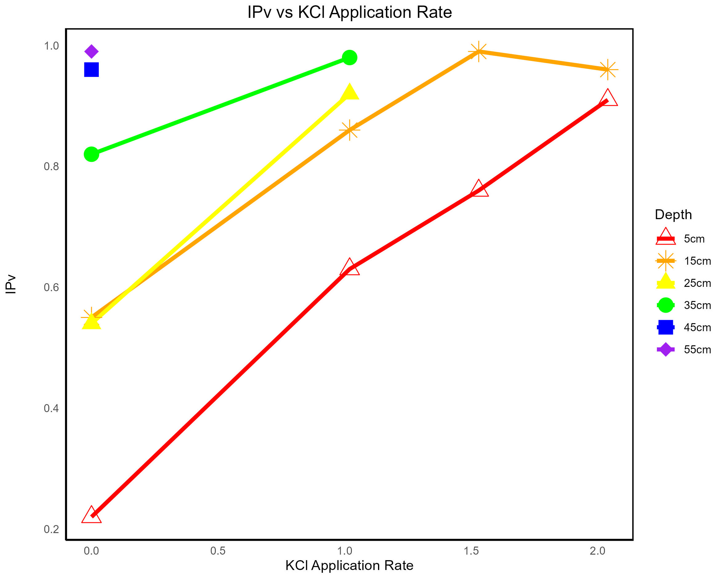
Figure 7 Inflection Point value (IPv) averaged per repetition in relation to the K (KCl) rate (0, 1.02, 1.52, and 2.04 kg/ha) at each sensor depth (5-55 cm).

While Figure 7 exhibited general increasing trends in IPv across all applications at both the 5 and 15 cm depths, Table 5 shows that the 5 cm depth was the only depth at which IPv increased at a significant rate as K application rate increased. At the 5 cm depth, each application rate was different from each other in addition to the control and display the ability for IPv to distinguish between application rates of K applied. The absence of IPv below the 15 cm depth could be attributed to the nature of the experimental design in our study, where a single water/nutrient application was performed per repetition. Although results were not significant for N, and P application rates and depths, IPv were observed up to the 35 cm depth for N, and across all depths for P. Future experiments should consider longer repetitions and more frequent watering to identify the sensitivity of sensors below 30 cm depth to nutrient availability.

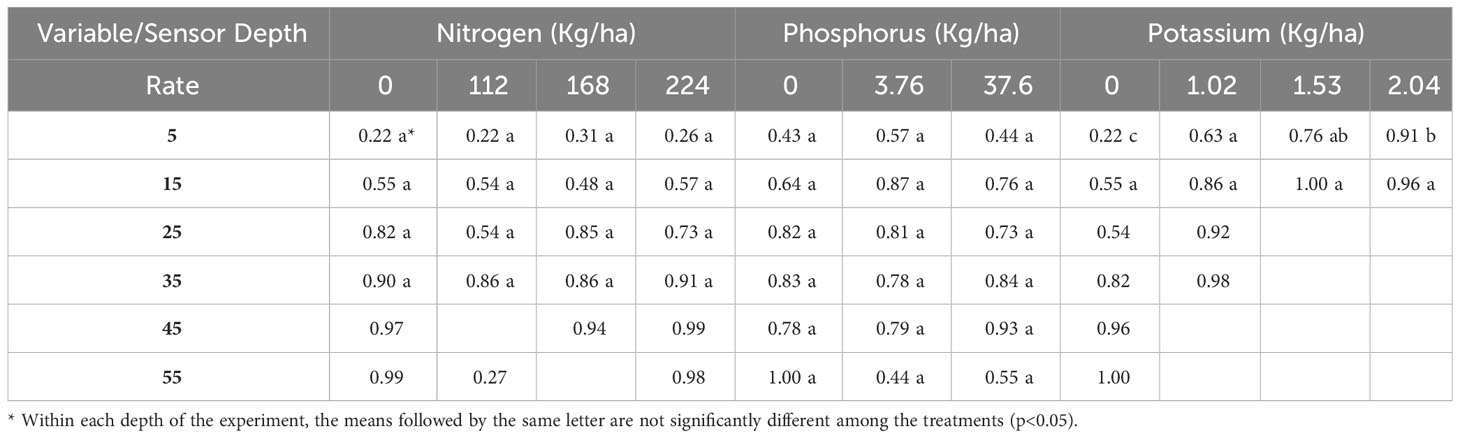
Table 5 ANOVA inflection point value means for N, P, and K treatments at each sensor depth (5-55 cm).

3.2.2 Time of inflection point occurrence

When comparing IPt at each depth within individual K application rates, there is a direct correlation between the increase in IPt and each application rate at depths 5 and 15 cm (Figure 8). At the 5 cm depth, IPt increases directly with the increased rate of K applications. At the 15 cm depth, there is an overall increase at application rate increases, with a slight decrease at the highest application rate. IPts only occur at the lowest application rates for 25 and 35 cm depths, and only occur within the control application at the 45 and 55 cm depths. Table 6 shows that only the SMS at the 5 cm depth shows significant increases in IPt across the K application rates. Similarly, each application rate had a higher IPt compared to the control and was significantly different from each other. This indicates IPt’s potential to detect differences in K concentration within the soil at the 5 cm depth after 24 hours post-application.

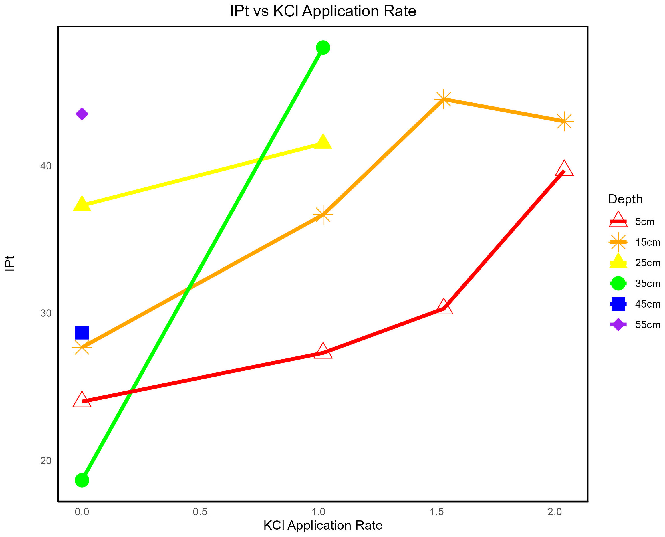
Figure 8 Inflection Point Time (IPts) averaged per repetition in relation to the K (KCl) rate (0, 1.02, 1.52, and 2.04 kg/ha) at each sensor depth (5-55 cm).

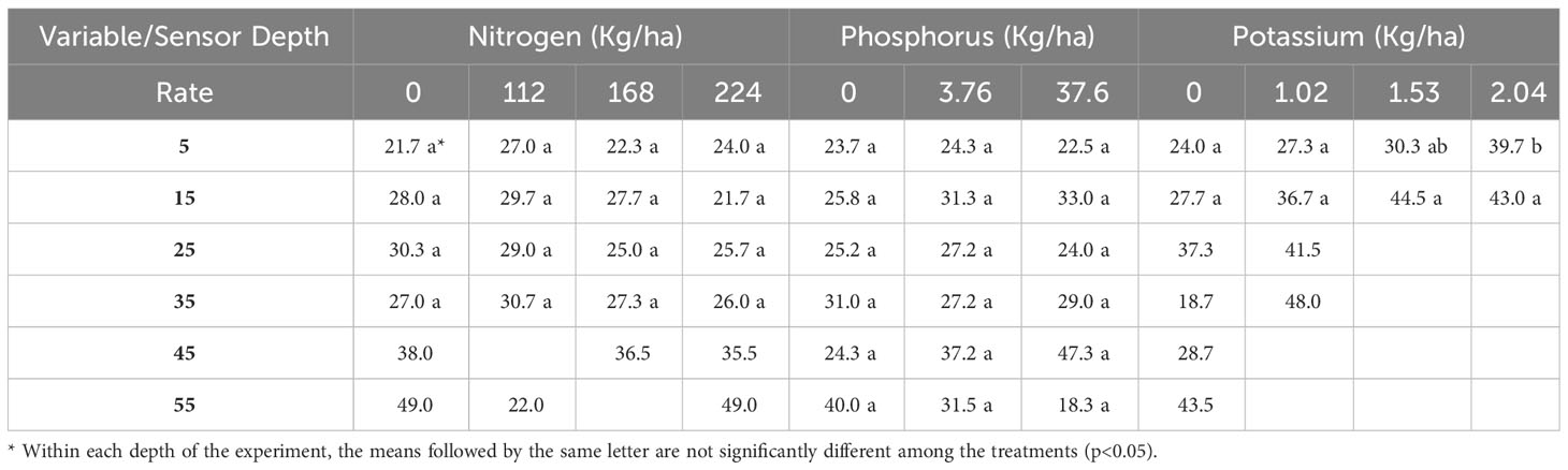
Table 6 ANOVA inflection point time means for N, P, and K treatments at each sensor depth (5-55 cm).

3.3 Convergence value

Table 7 shows no significant differences in the N and P experiments, while K yielded results indicating its detection through CV analysis. When comparing CVs across applications at each depth, there is a strong observable increase in CV as the K application rate increases within the 5 to 35 cm range (Figure 9). Unlike the MP and IP analysis, in each of the instances the increased application rate yielded an increased mean value CV down to the 35 cm depth. At the 45 and 55 cm depths, the CV maintains high both at the control and each K application treatment.

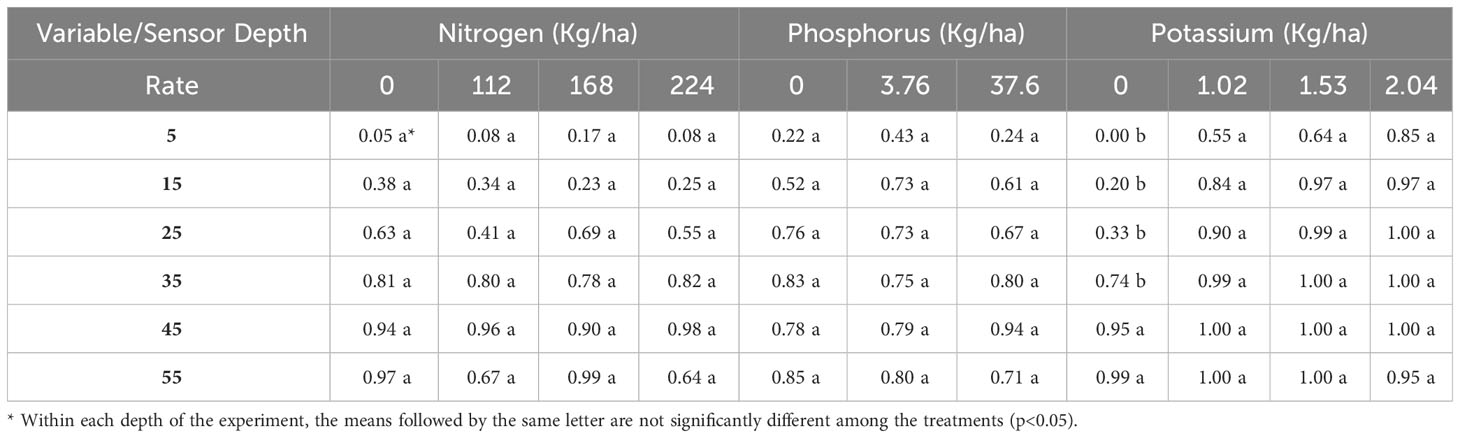
Table 7 ANOVA convergence value means for N, P, and K treatments at each sensor depth (5-55 cm).

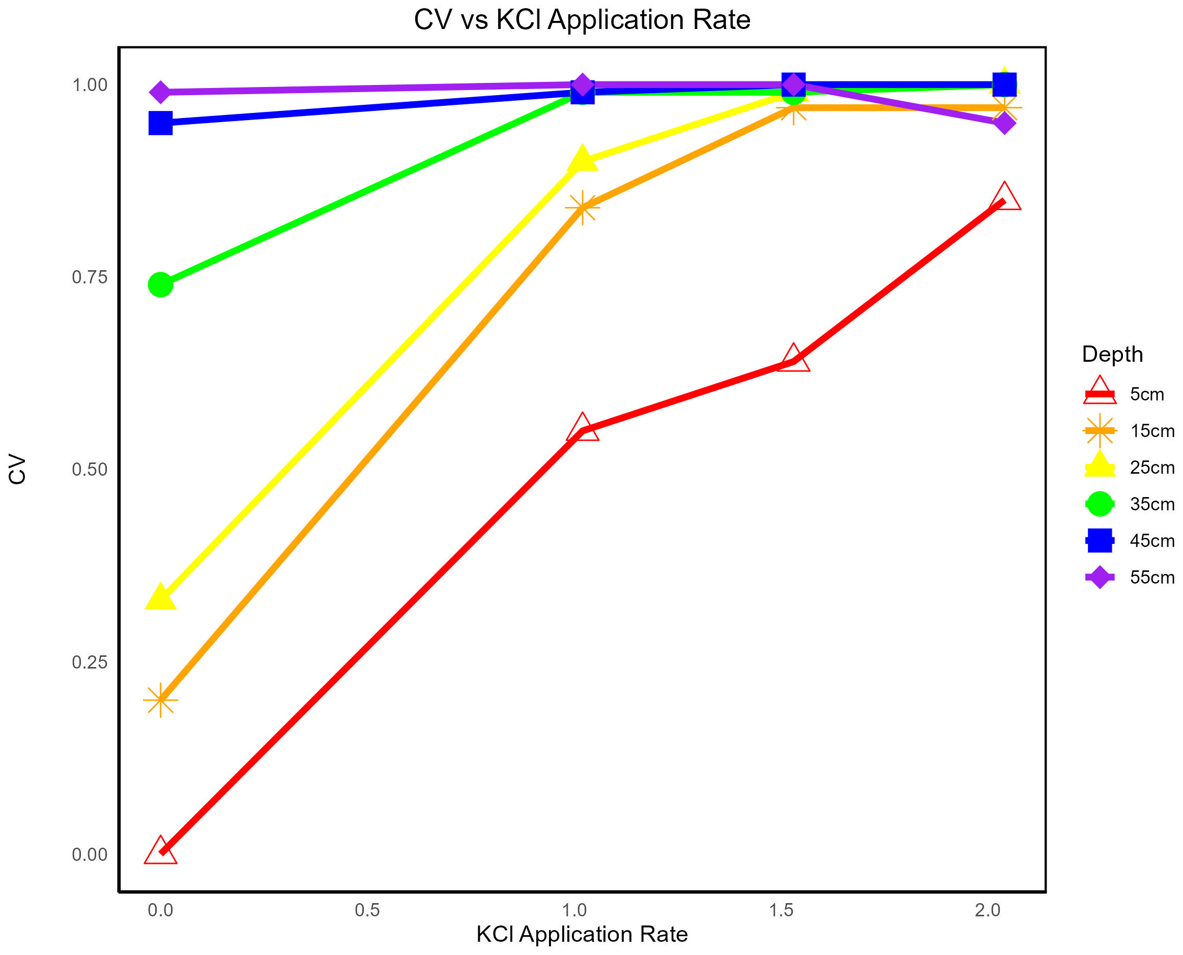
Figure 9 Convergence values (CVs) averaged per repetition in relation to the K (KCl) rate (0, 1.02, 1.52, and 2.04 kg/ha) at each sensor depth (5-55 cm). A direct correlation between CVs and application rate of KCl applied is observable.

From the surface down to 35 cm, the statistical comparison of CV between treatments showed that the SMP successfully distinguished each treatment from the control (Table 7). CVs did not distinguish between treatments however, and were only capable of detecting the presence or absence of K. The laboratory results are consistent with the CV findings were it was confirmed the presence of K from the soil surface down to 35 cm. A slight contrast found in the laboratory result was the identification that K was present down to the 40-50 cm depths, while difference in CV were not found across treatments at that level. Although there were not differences below the 35 cm depth, a pooling effect may have occurred due to the movement of water to the lower layers of the core. This might have influenced the VIC signals due to the presence of K in the solution.

3.4 Soil nutrient laboratory results

Table 4 suggests no significant difference in N rate throughout each sensor depth and each treatment, ranging from 0.05 – 0.103% TN. Laboratory analysis confirmed undetectable P concentrations for the control and low treatments. In the high treatment, P mostly remained in the top 20 cm of the soil core, with a smaller amount descending up to the 40 cm depth. K analysis suggests this nutrient was mobile, up to the 60 cm depth for the average and high treatments. Despite its mobility, mean values suggest the highest concentrations of K were mostly found at 20 and 30 cm depth for average and high treatments, respectively. The treatment and the SMS depth interaction results indicated significance for P (p-value = 1.12E-11), whereas the N (p-value = 0.883) and K (p-value = 0.778) displayed no significant interaction effects.

4 Discussion

4.1 VIC sensor values as indicators of nutrient presence in the soil profile

K’s presence in the soil and nutrient location can be determined by assessing MP, IP, and CV values from SMS readings. MPv was particularly successful at differentiating between the control and each application rate. In the topsoil layers, regardless of the application rate applied, MPv showed higher values than the control. IP was the most successful at distinguishing between application rates. Each application rate at the 5 cm mark had an increasing IPv and IPt as application rate increased. CV gave the strongest indication of whether K was present in the cores. While this method could not differentiate between application rates, CVs clearly increased in the presence of K at each rate. Related studies evaluating sensing conductance methods have found that sensor readings can be an indirect method to assess major nutrients in the soil (Eigenberg et al., 2002; Korsaeth, 2005).

MP measurements could be a good indicator for the development of real-time precision nutrient management systems. As more studies on conductance-based sensor development are produced (Basterrechea et al., 2020; Rocher et al., 2020), more information would be available for the development of robust decision-support systems related to the potential nature, concentration, or location of K within a field, after in-field sensor calibration is completed. Progress in the incorporation of in-field sensors for the indirect assessment of nutrients through fertigation are underway (Avşar and Mowla, 2022) and under development. This, along with the findings from this study, can contribute to a more practical and data-based in-field nutrient management.

While IP does not provide immediate results and is dependent on the CV, IP showed the best ability to distinguish between application rates and correlate them to K rates within the soil. MP from in-field SMPs and SMSs could be used as a real-time water saving parameter for nutrient management as this data is available, but underutilized. An increased or delayed MP during a fertigation event, when nutrients are applied through irrigation, would be an indicator of potentially increased K within the soil. This could determine how far down into the soil the K is moving and provide information to prevent nutrient leaching and environmental pollution in freshwater systems (Pathan et al., 2007). After such irrigation event occurs, as the soil begins to dry and IP and CV points are identified, IP could be used to quantify the concentration of K in the soil that may have been or was a risk of leaching, and CV used to finalize the resting place of the K after the event. This information would be useful in both identifying the movement of K in the soils during an irrigation event, as well as identifying the final location of K after the event. Furthermore, the nutrients in this experiment were studied separately but understanding the interactions between the nutrients, soil types and their combined effect of VIC is dynamic and should be studied to provide precise real time information to the end users.

The N and P control treatments at 55 cm have higher MPv, MPt, IPv, and IPt (Tables 2, 3, 5, 6) than the other treatments, potentially indicating an effect of the fertilizer presence on the moisture movement or a water cumulation effect. This scenario was not observed in K due to its high solubility nature compared to N and P and using pure sand as a medium, allowing more rapid nutrient movement (Table 4). The soil medium can influence sensor conductivity. Generally, the impacts of soil-water osmotic potential alterations are not considered for soil-water movement unless the solutes are in substantial amounts (Or and Wraith, 2002). However, in this study, this might have influenced the SMS readings. Masrie et al. (2017) developed and tested an optical transducer sensor for the detection of N, P, and K in soil, and found that soil characteristics in the presence of nutrients influence the frequency wavelength for sensor detection. This study suggest that SMSs require voltage thresholds that variates based on the nutrient assessed. Laboratory results confirmed that P was primarily present in the top 20 cm of the cores, yet despite statistical analysis comparing MPv, MPt, IPv, IPt, and CVs no significant differences were observed.

Our results-keeping in mind this study only tested one form of each element in a pure sand soil type-suggest that the SMP primarily detects K ions from the fertilizers applied and can be used as part of currently available irrigation scheduling decision support systems (DSS). Several methods of combining irrigation sensing technology with soil moisture prediction models (Kashyap and Kumar, 2021) and DSSs (Rinaldi and He, 2014) are available. Any variation in the MP, IP, or CV could indicate potential K presence in the soil. However, this signal variation could also originate from other ions in the soil with a sufficiently strong osmotic potential. Although the interactions between N, P, and K when combined has yet to be explored, such interactions could potentially enhance their VIC signals.

5 Conclusion

This study demonstrated that the SMPs’ VIC readings have the ability to detect K within the soil profile and provide an indication of its rate and location. The statistical analysis from MP, IP, and CV from 24-hour VIC readings has proven to be an effective method for K detection. While our study did not yield significant results for N and P, mean value comparison hints at the potential for detection, possibly through other indirect methods, or different forms of N and P that yield strong VIC in soil. The results from this study can serve as a foundation for implementing fertigation management programs, focusing on water and K movement in the soil, and indirectly managing N and P by maintaining water within the effective root zone depth for crops. Future work should investigate temperature differences related to in-field seasonal patterns. Utilizing IP as a way of differentiating nutrient concentrations showed great promise at the 10 cm depth. Overall, integrating nutrient management strategies into existing agricultural technologies, such as the SMPs investigated in this study, is crucial to accelerating the adoption of precision agriculture technology in practical applications within the agricultural industry.

Data availability statement

The raw data supporting the conclusions of this article will be made available by the authors, without undue reservation.

Author contributions

ZS: Writing – review & editing, Data curation, Formal analysis, Investigation, Methodology, Project administration, Software, Writing – original draft. AA: Data curation, Formal analysis, Investigation, Methodology, Software, Writing – original draft. SG: Conceptualization, Funding acquisition, Resources, Supervision, Writing – review & editing.

Funding

The author(s) declare financial support was received for the research, authorship, and/or publication of this article. This study was funded by the Science and Technologies for Phosphorus Sustainability (STEPS) Center, a National Science Foundation Science and Technology Center (CBET-2019435).

Acknowledgments

The authors would like to acknowledge Daniel Palacios-Linares for his assistance in data collection. Special thanks to the reviewers for their valuable comments that helped improve the paper.

Conflict of interest

The authors declare that the research was conducted in the absence of any commercial or financial relationships that could be construed as a potential conflict of interest.

Publisher’s note

All claims expressed in this article are solely those of the authors and do not necessarily represent those of their affiliated organizations, or those of the publisher, the editors and the reviewers. Any product that may be evaluated in this article, or claim that may be made by its manufacturer, is not guaranteed or endorsed by the publisher.

References

Avşar E., Mowla M. (2022). Wireless communication protocols in smart agriculture: A review on applications, challenges and future trends. Ad Hoc Networks 136, 102982. doi: 10.1016/j.adhoc.2022.102982