Ipomoea cairica (L.) from Mangrove Wetlands Acquired Salt Tolerance through Phenotypic Plasticity
Figure 1.
The growth of different ecotypes of Ipomoea cairica under salt stress that shows the phenotypic adaptability of the coastal ecotype to salt stress. (A,B) Root growth after 2 weeks of hydroponics, including (A) the morphology of the root (Bar = 1 cm) and (B) root length. (C–F) The growth trend of the two ecotypes within 60 d after transplantation, including (C) the main stem length. (D) Leaf number during the salt treatment. (E) Branch number. (F) Flower number. All the data represent the mean ± SE. The different letters in the bar graphs indicate significant differences at p < 0.05. SE, standard error.
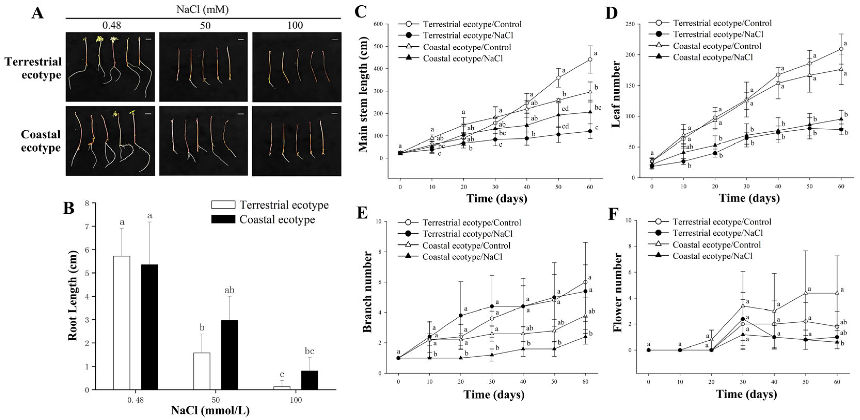
Figure 2.
Effect of 150 mmol/L NaCl on the growth of terrestrial ecotype and coastal ecotype of Ipomoea cairica (A–D) after 60 d. (E) Fresh weight of the roots. (F) Fresh weight of the aboveground biomass. (G) Fresh weight of the total biomass. (H) Root/shoot ratio. All the data represent the mean ± SE. Different letters indicate a significant difference at p < 0.05. SE, standard error.
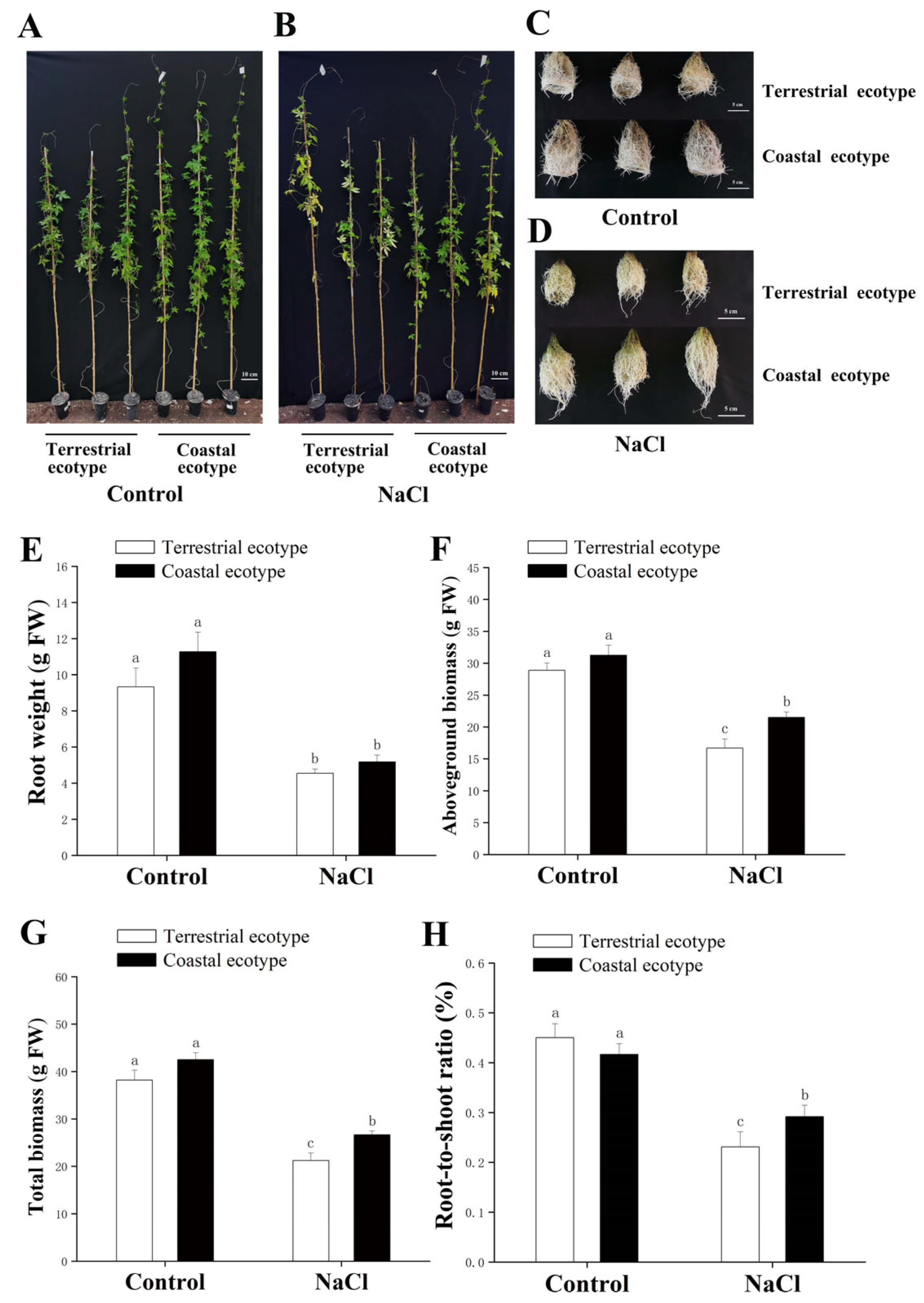
Figure 3.
The terrestrial ecotype suffered more severe cellular damage under salt stress than the coastal ecotype. (A,B) Apoptosis of the protoplasts under the salt treatment detected by Annexin V-FITC/PI double staining flow cytometry. (A) Flow cytometric estimation of apoptosis. (B) Representative flow cytometry histograms of the apoptosis. (C,D) Root cell membrane integrity detected by Evans blue staining. A darker stain, lower integrity. (C) Dead cells that were stained blue. (D) The degree of damage to the cell membrane. (E) Malondialdehyde (MDA). (F) Relative electrical conductivity (REC). (G) Leaf relative water content. Bar = 1 μm. All the data represent the mean ± SE. The different letters in the bar graphs indicate significant differences at p < 0.05. SE, standard error.
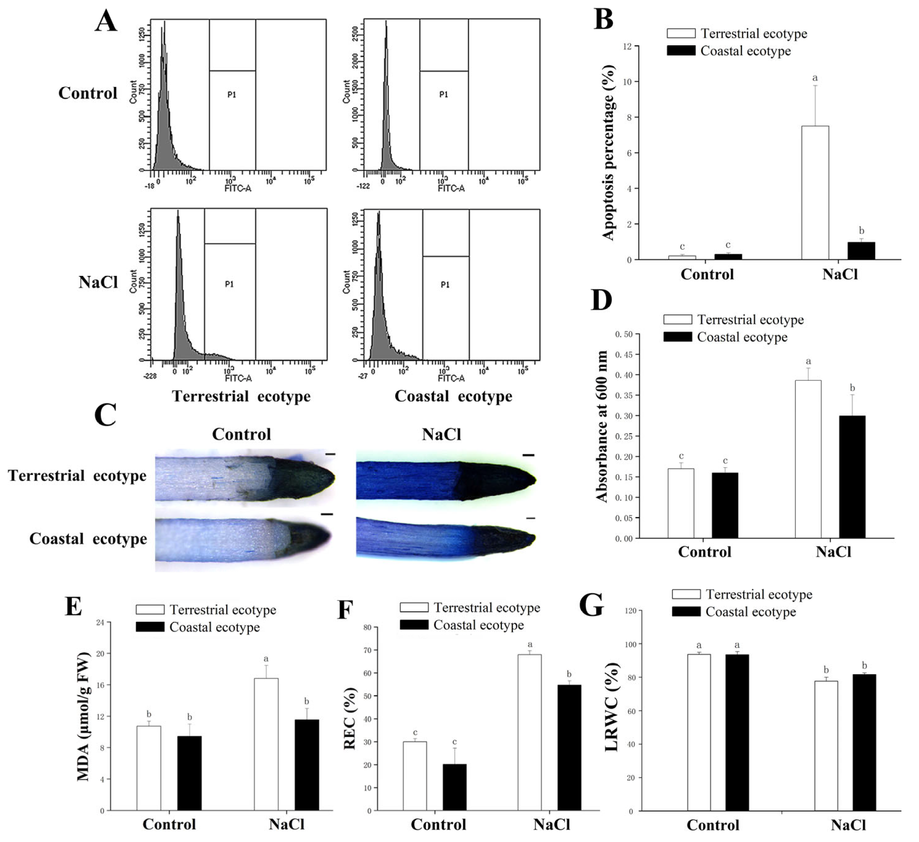
Figure 4.
Physiological changes induced by salt in Ipomoea cairica leaves. (A) Anthocyanin content. (B) Superoxide dismutase (SOD). (C) Peroxidase (POD). (D) Catalase (CAT). All the data represent the mean ± SE. The different letters in the bar graphs indicate significant differences at p < 0.05. SE, standard error.
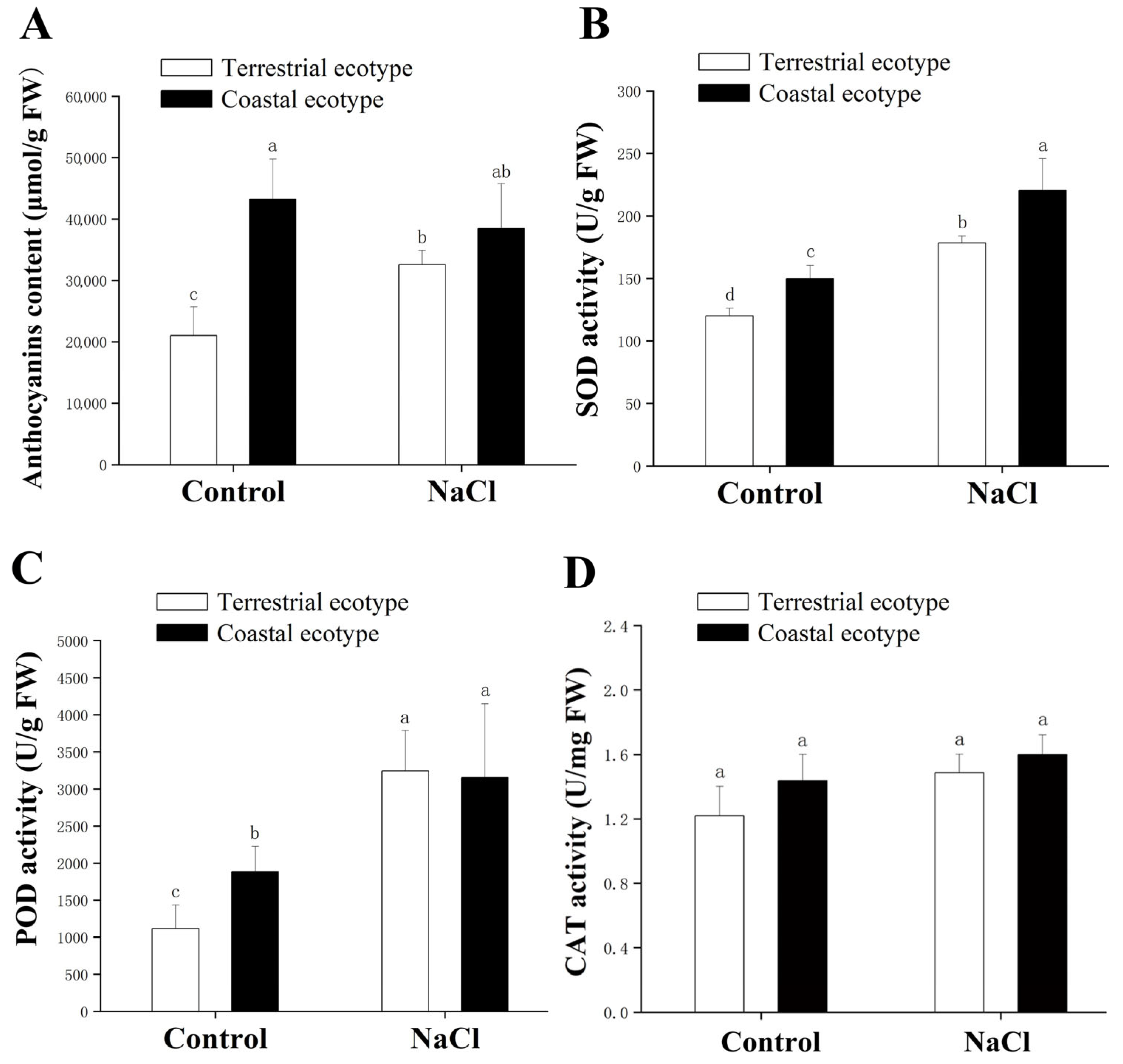
Figure 5.
Effect of NaCl concentrations on the salt glands of the two ecotypes after 60 d. (A–D) Salt glands, red arrows. (E) Salt gland area. (F) Number of salt glands. (G) Salt gland density. All the data represent the mean ± SE. The different letters in the bar graphs indicate significant differences at p < 0.05. SE, standard error.
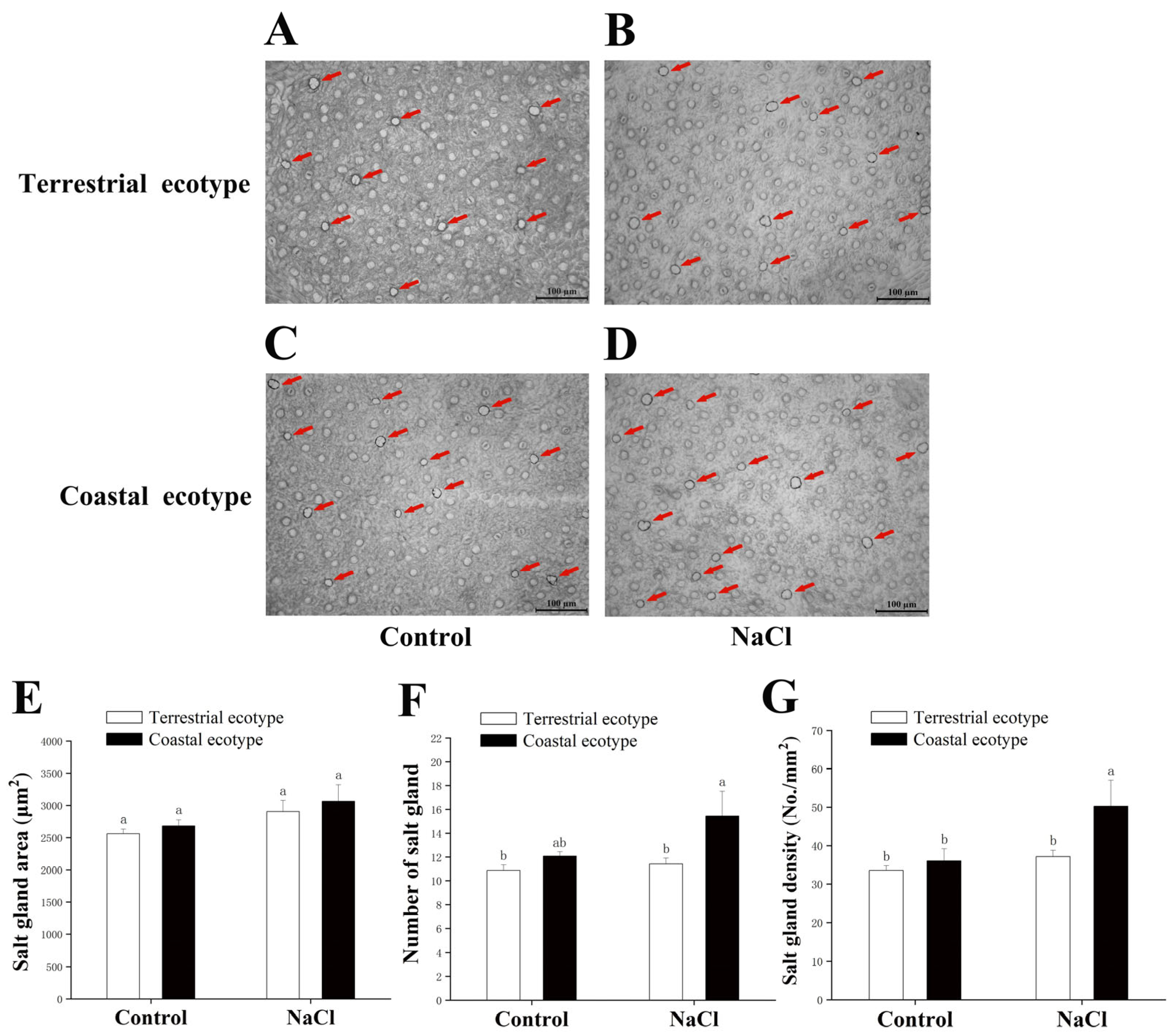
Figure 6.
The contents of elements and their allocations in the roots, stems, and leaves of the coastal ecotype were more balanced and conducive to growth than those of the terrestrial ecotype under salt stress. (A) Content of sodium ion (Na+). (B) Content of potassium ion (K+). (C) K+: Na+ ratio. (D) Content of nitrogen (N). (E) Content of phosphorus (P). (F) N: P ratio. All the data represent the mean ± SE. The different letters in the bar graphs indicate significant differences at p < 0.05. SE, standard error.
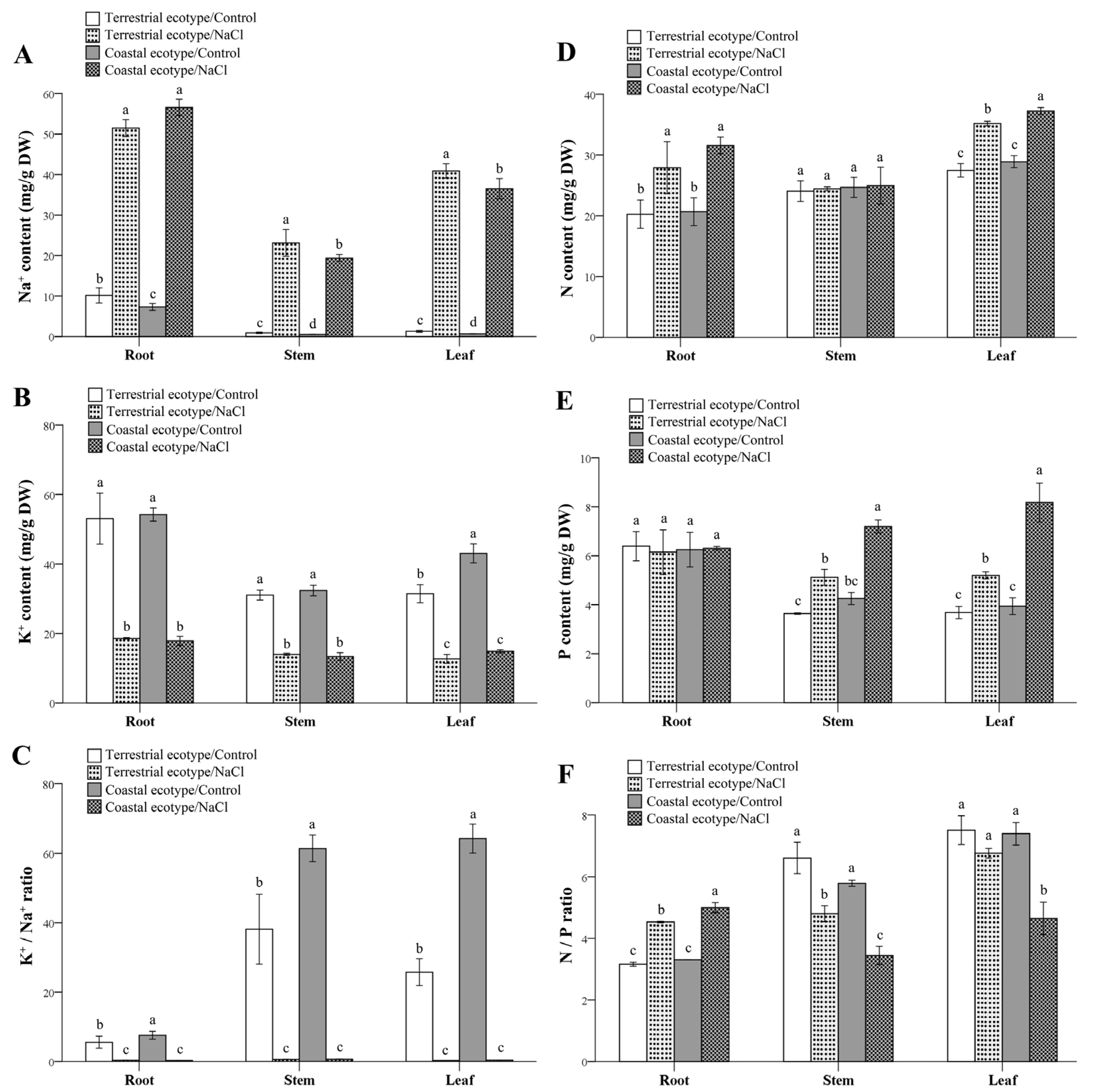
Figure 7.
Effect of NaCl concentrations on the stomata and proline content of the two ecotypes after 60 d. (A–D) Stomata. (E) Number of stomata. (F) Stomatal density. (G) Proline. All the data represent the mean ± SE. The different letters in the bar graphs indicate significant differences at p < 0.05. SE, standard error.
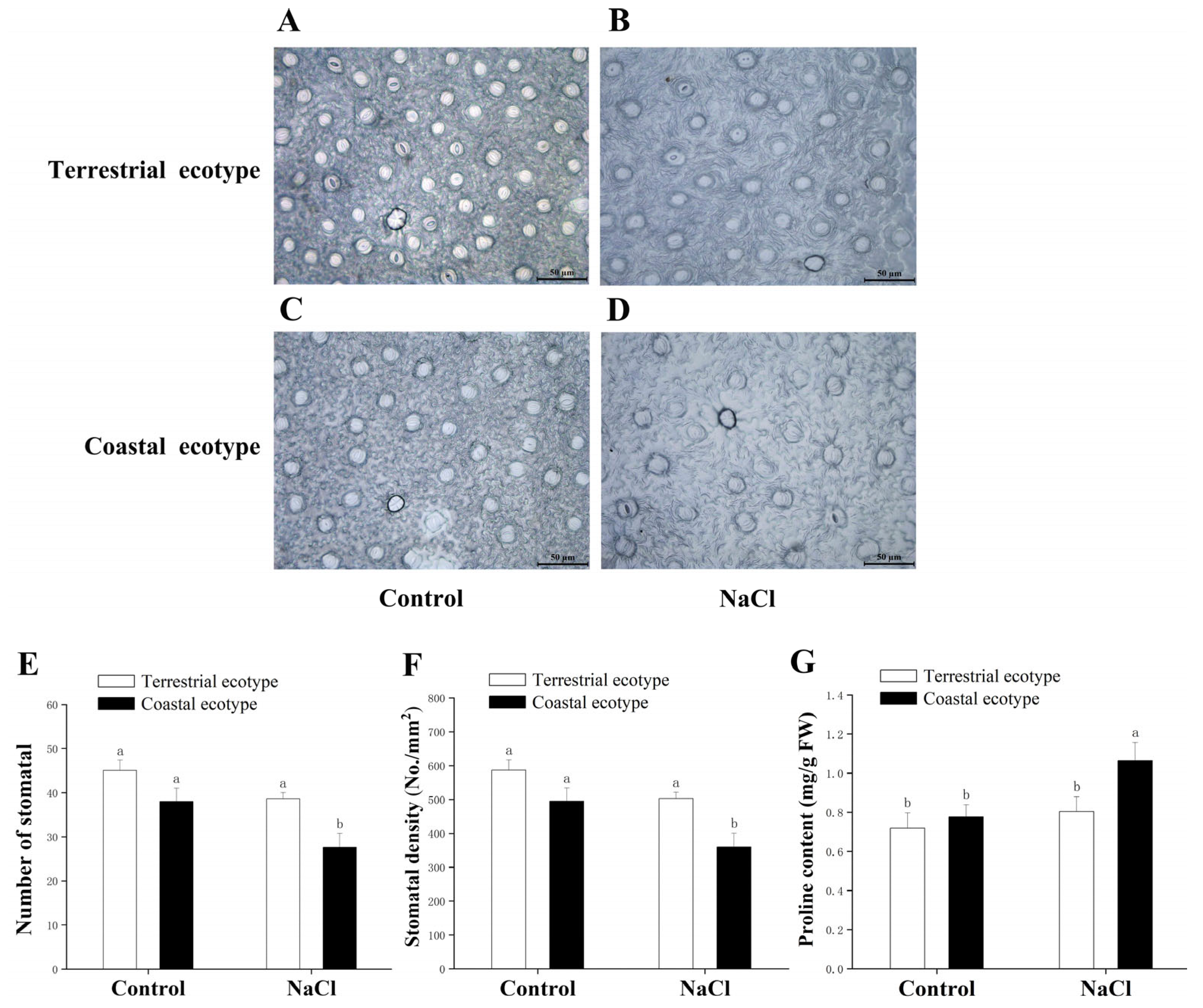
Figure 8.
The chlorophyll content and chlorophyll fluorescence parameters of the two ecotypes under salt stress. (A) Total chlorophyll (chl a + b). (B) Chlorophyll a. (C) Chlorophyll b. (D) Chlorophyll a/b. (E) Maximal efficiency of PSII photochemistry. (F) Actual quantum yield of PSII. (G) Photochemical quenching coefficient. (H) Non-photochemical quenching coefficient. (I) Electron transport rate. PSII, photosystem II. All the data represent the mean ± SE. The different letters in the bar graphs indicate significant differences at p < 0.05. SE, standard error.
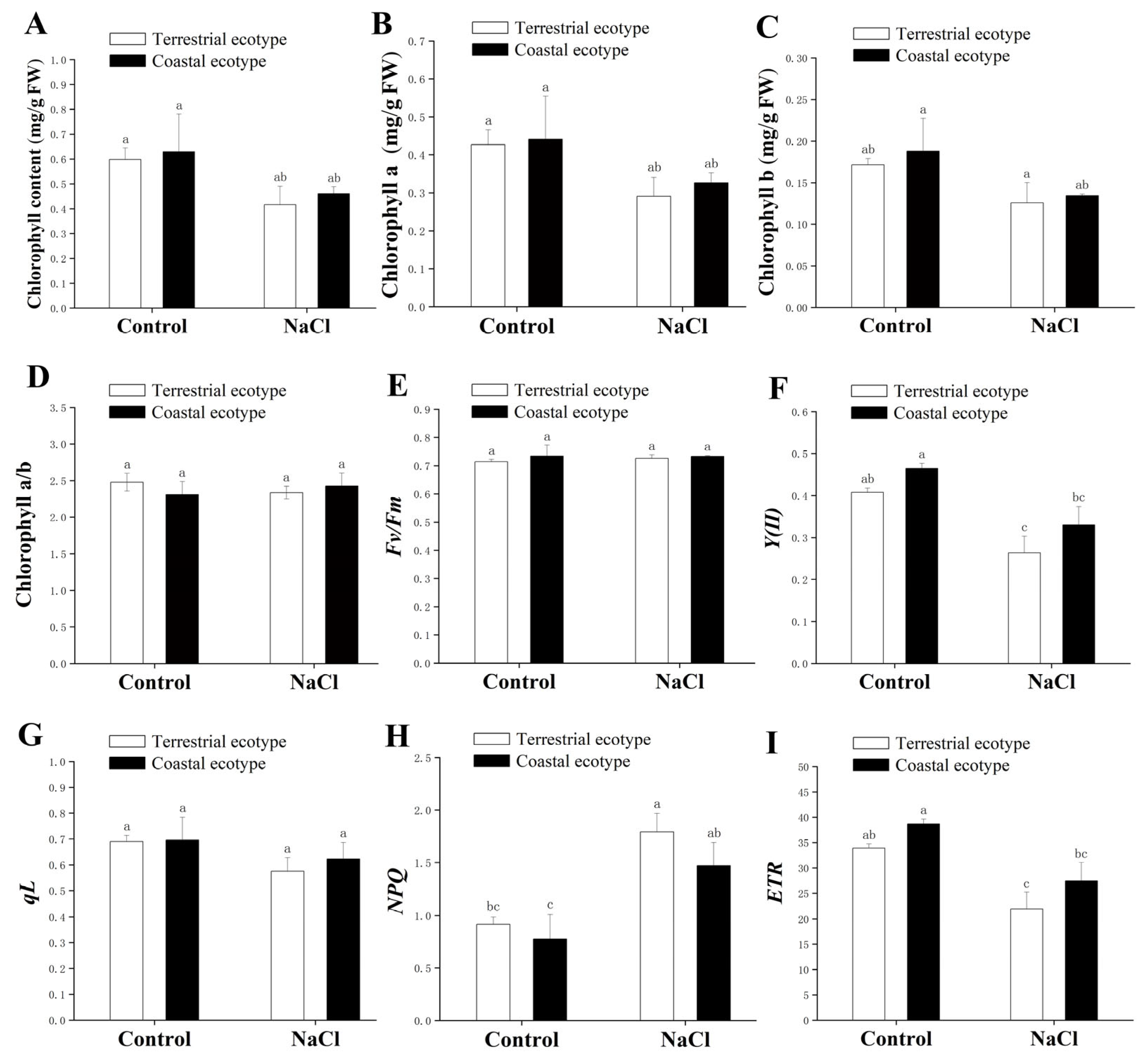
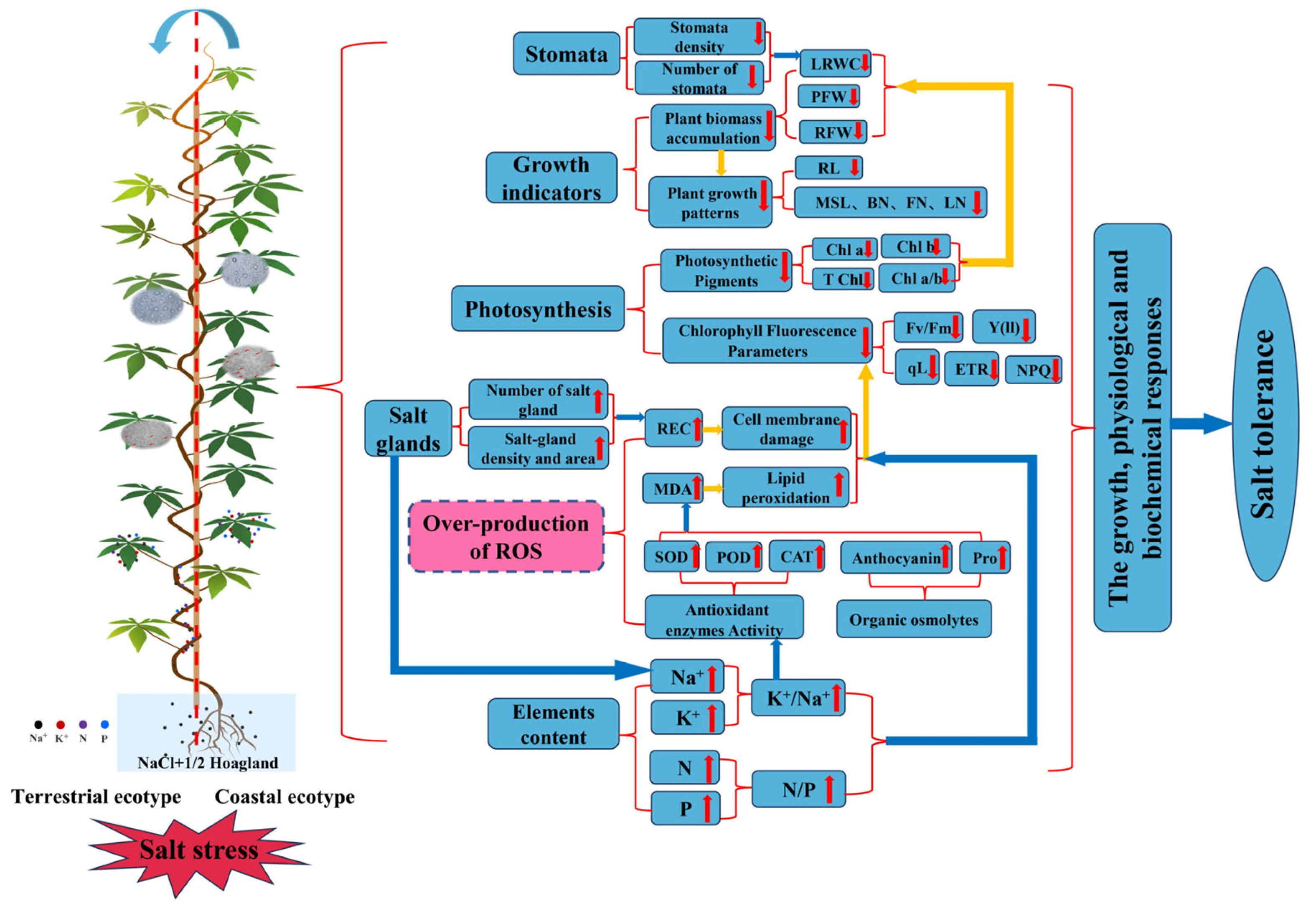
Figure 9.
Schematic representation of the inhibition of growth induced by salinity. LRWC, leaf relative water content; PFW, plant fresh weight; RFW, fresh weight of roots; RL, root length; MSL, main stem length; BN, branch number; FN, flower number; LN, leaf number; Chl a, chlorophyll a content; Chl b, chlorophyll b content; TChl, total chlorophyll content; Chl a/b, chlorophyll a/b; Fv/Fm, maximal efficiency of PSII photochemistry; qL, photochemical quenching coefficient; Y(ll), actual quantum yield of PSII; NPQ, non-photochemical quenching coefficient; ETR, electron transport rate; MDA, malondialdehyde; REC, relative electrical conductivity; Pro, proline; SOD, superoxide dismutase; POD, peroxidase. PSII, Photosystem II; Na+, sodium ion; K+, potassium ion; K+/Na+ sodium and potassium ion ratio; N, nitrogen; P, phosphorus; N/P, nitrogen and phosphorus ratio.