Automation and Robots for Disaster Response

MOLM: Alleviating Congestion through Multi-Objective Simulated Annealing-Based Load Balancing Routing in LEO Satellite Networks

By inergency On Mar 25, 2024

[ad_1]

1. Introduction

Satellite internet, as a communication network with extensive coverage and high flexibility, is gradually becoming a crucial means of global connectivity. However, due to its unique communication characteristics and resource constraints, satellite internet often faces challenges of load imbalance when confronted with large-scale user demands. Optimizing load balance is essential for improving the performance of satellite internet and reducing communication latency. While load balancing issues have been extensively researched and applied in traditional ground communication networks, the peculiarities of satellite internet make this problem more complex and challenging.

The core of the load balancing problem lies in the proper allocation of communication loads within the satellite internet system, ensuring the maximization of resource utilization for each satellite node to enhance overall communication efficiency. However, factors such as an uneven geographical distribution of satellite nodes, variability in satellite conditions, and resource limitations pose constraints on the applicability of traditional load balancing strategies in satellite internet.

To address the load balancing issue in satellite internet, many strategies use the latency of new paths as an evaluation metric without considering path stability. However, path stability is also an important factor, as the dynamics of satellite networks and satellite movements can lead to path switching, resulting in switching and routing maintenance costs. Choosing a path with high stability can reduce costs. This paper proposes a low-maintenance, cost–load balancing routing method based on the multi-objective simulated annealing algorithm, named MOLM. Simulated annealing, as a heuristic optimization algorithm, possesses global search capabilities and adaptability to multi-objective optimization problems. When network congestion occurs, a continuous neighbor set is established, and the multi-objective simulated annealing algorithm is used to select neighboring satellites that satisfy both strong path stability and low latency to replace congested nodes, thereby improving the overall performance of the satellite internet system.

The main contributions of the paper are embodied in the following aspects. (1) Based on the predictability of satellite networks, the concept of a continuous neighbor set is proposed, which includes nodes that can maintain continuous connections with the predecessor and successor of congested nodes. (2) The MOLM algorithm is used, which employs the multi-objective simulated annealing (MOSA) framework to iteratively derive an optimal element from the continuous neighbor set to replace congested nodes within a specific path, generating the final solution aimed at alleviating network congestion. (3) A comprehensive comparative experiment is conducted to demonstrate the performance of the MOLM algorithm, including comparative experiments under different networking methods and varying satellite constellation densities. Finally, the reliability of FRR-BP is measured using the time taken to reconstruct backup paths.

The rest of the paper is organized as follows. In Section 2, we summarize the work related to satellite network congestion resolution strategies. In Section 3, we introduce the architecture of satellite networks. In Section 4, we first introduce the process of using the MOLM algorithm to address network congestion issues. Then, we introduce the Fast Rerouting mechanism based on backup paths (FRR-BP). In Section 5, a comprehensive comparative experiment is conducted to demonstrate the performance of the MOLM algorithm. In Section 6, we give the conclusion.

4. Algorithm Design

4.1. Overview of the MOLM Algorithm

The overview of the MOLM algorithm is shown in Figure 2. First, it will generate the initial solution using a shortest path algorithm like Dijkstra’s algorithm. Dijkstra’s algorithm will find paths with the minimum latency, but they are often accompanied by network congestion and path instability. Second, it will check for network congestion using Algorithm 1. If congestion occurs, it will establish the continuous neighbor set using Algorithm 2. Third, it will iterate by employing the multi-objective simulated annealing framework, with the minimum temperature and maximum iteration count as constraints. During each iteration, it will randomly select an element from the continuous neighbor set and replace the congested node to generate a new solution. Then, it will compare the new solution with the initial solution. If the new solution is better, it will accept it directly. If the initial solution is better, it will accept the new solution with a certain probability P, and with probability 1 − P, it will stick to the initial solution. Finally, it will provide a routing solution to address network congestion.

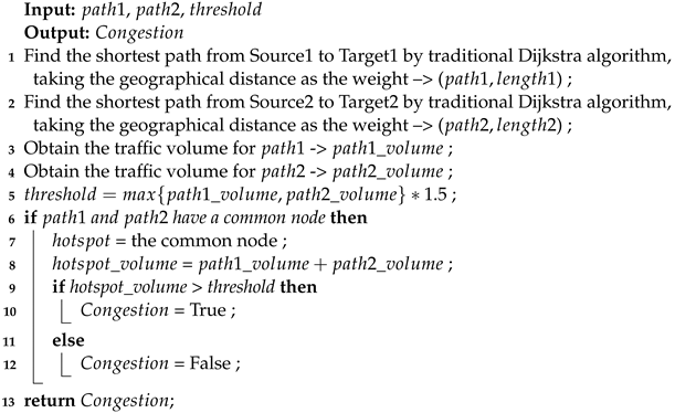
4.2. Judgment of Network Congestion

Assuming there are two services, each with one path, as shown in Figure 1 with corresponding red and blue colors, if both of these service paths pass through a certain satellite node, then this satellite node becomes a hotspot. Calculate the total traffic at the hotspot, and if the total traffic exceeds the threshold, congestion is considered to have occurred. Regarding the threshold setting, we typically set it to 1.5 times the highest traffic volume in the service paths. The judgment of network congestion is depicted in Algorithm 1.

Algorithm 1: Judgment of Network Congestion

4.3. Establishment of the Continuous Neighbor Set

If congestion occurs, we use the MOLM algorithm to resolve the congestion. Before that, we need to establish a continuous neighbor set, which includes nodes that can maintain continuous connections with both the predecessors and successors of the congested node. The process of establishing the continuous neighbor set can be described using Algorithm 2.

Assuming the paths for Service 1 and Service 2 are [‘1’,‘2’,‘3’,‘6’] and [‘4’,‘5’,‘3’,‘7’]. The traffic volumes for path 1 and path 2 are 20 and 15, respectively. Therefore, the threshold is equal to 20 × 1.5 = 30. If both paths traverse satellite node 3 with cumulative traffic exceeding the threshold, network congestion occurs, with node 3 identified as the congested node. To alleviate this congestion, we intend to modify the path of Service 2. The predecessor and successor nodes for this congestion are nodes 5 and 7, respectively.

Algorithm 2: Establishment of the Continuous Neighbor Set

To obtain the nodes that can maintain continuous connections with both node 5 and node 7, we need to know the nodes that are adjacent to nodes 5 and 7 at the current time as well as the nodes that will remain adjacent to nodes 5 and 7 after a certain period. Therefore, we require the adjacency matrix of the satellite nodes at the current time and after a certain period. Figure 3a represents the adjacency matrix of satellite nodes at the current time t, while Figure 3b represents the adjacency matrix of satellite nodes at time

t + Δ t

Therefore, the nodes adjacent to nodes 5 and 7 at the current time t can be represented as $a_{5}$ = {1,0,1,0,0,1,1} and $a_{7}$ = {1,0,0,1,1,1,0}, and the nodes adjacent to nodes 5 and 7 at time $t + Δ t$ can be represented as $b_{5}$ ={1,0,1,1,0,1,0} and $b_{7}$ = {1,1,0,1,0,1,0}. Let P = ( $a_{5} \cap b_{5}$ ) ∩ ( $a_{7} \cap b_{7}$ ) = {1,0,0,0,0,1,0}, where P represents the continuous neighbor set. The nodes in the continuous neighbor set are node 1 and node 6.

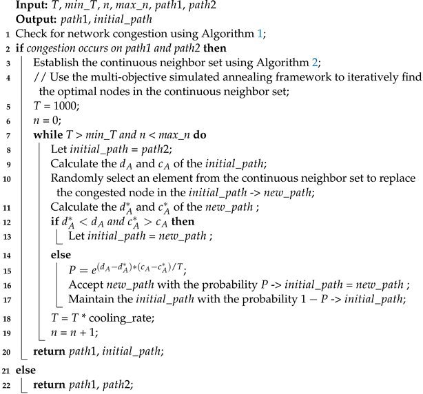
4.4. The Design of MOLM

The MOLM algorithm first checks for network congestion using the method shown in Algorithm 1. Second, if congestion occurs, it uses the method shown in Algorithm 2 to establish the continuous neighbor set. Last, MOLM will select an element from the persistent neighbor set to replace congested nodes. The MOLM algorithm employs the multi-objective simulated annealing (MOSA) framework to iteratively select the optimal nodes from the continuous neighbor set to replace congested nodes. During each iteration, a random element is selected from the continuous neighbor set to replace the congested node, generating a temporary new path as a new solution. The stability and latency of the new path are compared with those of the original path. If the new solution is superior to the original one, it is accepted directly. If the new solution is worse than the original one, it is accepted with a certain probability. The algorithm of MOLM can be described using Algorithm 3. The argument T means the temperature at the current moment, and

m i n_{T}

means the minimum temperature. The argument n means the number of iterations, and

m a x_{n}

means the maximum number of iterations. When the temperature reaches the minimum temperature or the number of iterations reaches the maximum number of iterations, the iteration will stop.

Algorithm 3: MOLM

From line 2 to line 7 in the MOLM algorithm, we show that it solves the congestion problem with dual optimization objectives related to path stability and latency, which are described as maximizing the average path duration and minimizing the average latency. The mathematical model of the multi-objective optimization problem is expressed as

$f : L \to \{\begin{matrix} min d_{A} \\ max c_{A} \end{matrix}$

(1)

In the given context, where f is the optimization objective function,

L = [l_{i j} [t]]

i, j = 1, 2, 3, 4 \dots N

L = [l_{i j} [t]]

represents the link from the starting point i to the ending point j at time t, where

d_{A}

is the average latency of these paths and

c_{A}

is the average duration of these paths. The constraints for establishing a link are as follows:

$\begin{matrix} v_{i j} & \in {0, 1}, \forall i, j \end{matrix}$

(2)

$\begin{matrix} v_{i j}^{*} & \in {0, 1}, \forall i, j \end{matrix}$

(3)

$\begin{matrix} v_{i j} & \geq l_{i j}, \forall i, j \end{matrix}$

(4)

$\begin{matrix} v_{i j} & = v_{j i}, \forall i, j \end{matrix}$

(5)

In the given context, Equations (2) and (3) involve

v_{i j}

and

v_{i j}^{*}

, representing whether satellite i and satellite j are visible and continuously visible, respectively. When visible,

v_{i j}

takes the value of 1; otherwise, it is 0. When continuously visible,

v_{i j}^{*}

takes the value of 1; otherwise, it is 0. Equation (4) indicates that a link between two satellite nodes can only be established if they are in a visible state. Equation (5) represents the symmetry constraint.

4.5. Fast Rerouting Mechanism

Fast Reroute (FRR) is a network fault recovery technique. In satellite networks, FRR can be implemented using either backup paths or local repair mechanisms. In the backup path-based FRR mechanism, when the primary path fails, data traffic is switched to the backup path. On the other hand, the local repair-based FRR mechanism involves computing multiple local paths to quickly repair the route near the point of failure. In this paper, we adopt the backup path-based Fast Reroute mechanism (FRR-BP) in the satellite network. In FRR-BP, when a node in the satellite network fails, the network control center removes the failed node from the network topology and recalculates the backup path from the source to the destination. To ensure the stable operation of the satellite network, it is essential to trigger the recalculation of the backup route and swiftly switch to the backup path when a network failure occurs, minimizing the impact of network failures on service quality and reliability. The details of FRR-BP are presented in Algorithm 4. Additionally, it is crucial to be mindful of potential network congestion when employing backup paths. If congestion occurs in the network, the resolution of congestion still necessitates the use of the MOLM algorithm.

Algorithm 4: Fast Rerouting Method Based on Backup Paths (FRR-BP)

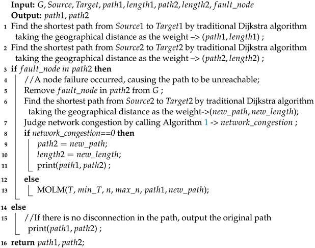5. Simulation Experiment Evaluation

5.1. Simulation Environment

We utilized the SILLEO-SCNS simulator proposed by B. S. Kempton [16], which is a simulation tool designed for studying routing in large-scale satellite networks. This tool enables the simulation of various satellite network architectures and routing schemes, allowing for performance evaluation. The architecture of this simulator primarily consists of a graphical user control interface, constellation class, and simulation class, as shown in Figure 4. The constellation class serves as the core component responsible for generating satellites, ground stations, and network structures. The simulation class handles the visualization of the satellite network and all associated animations. The GUI provides a user control interface that allows users to configure constellation parameters, set the source and destination for path planning, and specify satellite connectivity options. Communication between the GUI and simulation is facilitated through interprocess communication for information exchange.

The simulation adopts a Walker constellation configuration of 100/10/1, with an orbit altitude of 1200 km and an orbital inclination of 60°. To facilitate analysis and calculations, the sampling period for the constellation data is set to 10 s. The setting of simulation parameters is shown in Table 2. In the temperature cooling schedule for multi-objective simulated annealing, the initial temperature is set to 1000 °C. Following Kirkpatrick et al.’s analysis, the Boltzmann constant during temperature cooling is set to 0.95. The iteration limit is set to 2500, and the iteration stops when the temperature cools to the minimum temperature or the iteration count reaches the upper limit.

5.2. Benchmarking Algorithms and Complexity Analysis

Our proposed MOLM algorithm aims to address network congestion issues, and we analyze its complexity in this part. The core idea of the MOLM algorithm is to establish a continuous neighbor set during network congestion and then utilize a multi-objective simulated annealing framework to select the best node from this set to replace congested nodes, achieving the goals of avoiding congestion while maintaining path stability and low latency.

$O p t i m u m$ is based on a greedy algorithm for node replacement. It employs a greedy strategy to select nodes from the continuous neighbor set, optimizing path stability and latency of the entire path. The strategy of $S h o r t e s t$ $P a t h$ generates the shortest path for congested traffic in the network, aiming to minimize latency. The difference between the two is that $O p t i m u m$ selects one node from a limited number of nodes, namely those in the continuous neighbor set, to minimize latency. Meanwhile, the shortest path algorithm searches for a route from $S o u r c e$ to $T a r g e t$ , resulting in the globally minimal latency path.

Firstly, we discuss the complexity of the MOLM algorithm. For the filtering process of the continuous neighbor set, we note that its time complexity is approximately O(n), where n represents the cardinality of the continuous neighbor set. Similarly, for the selection of the best node, we employ the Optimum method based on a greedy algorithm, with a time complexity that is also approximately O(n). This is because, under the greedy strategy, selecting nodes from the continuous neighbor set is a relatively efficient operation.

Furthermore, the complexity of the shortest path algorithm is also discussed. We use the Dijkstra algorithm to find the shortest path. Due to the +Grid networking method employed, with each satellite maintaining four connections, the topology graph is relatively sparse. Therefore, its time complexity is approximately O(nm), where m represents the number of edges in the network.

In summary, the MOLM algorithm exhibits low time complexity in addressing network congestion issues, making it capable of efficient operation in practical applications and effectively enhancing network performance.

5.3. Simulation Result

We measure path stability using the average duration of a path, which is calculated based on the consecutive occurrences of a particular path. Assuming a path persists continuously for N times, the duration of that path would be

N * s t e p

. The comparison of different algorithms is shown in Figure 5.

In terms of path stability, when using a shortest-path-first rerouting mechanism to address network congestion, the average path duration is approximately 125 s. By employing the MOLM algorithm in conjunction with multi-objective simulated annealing to address congestion, the average path duration can exceed 225 s. This represents an improvement of around 80% compared to the $S h o r t e s t$ $P a t h$ strategy.

In terms of path latency, the

S h o r t e s t

P a t h

strategy achieves minimal latency, approximately around 70 ms. The MOLM algorithm filters out the continuous neighbor set from all satellites, iteratively selects an optimal candidate neighbor using multi-objective simulated annealing, and replaces congested nodes. This strategy, while enhancing path stability, maintains a relatively small latency cost. As shown in Figure 5b, the latency introduced by MOLM is around 80 ms, an increase of less than 15% compared to

S h o r t e s t

P a t h

This is because the $S h o r t e s t$ $P a t h$ strategy prioritizes the selection of the shortest path, sacrificing path stability in pursuit of minimizing latency. In contrast, the nodes selected by the MOLM algorithm in the continuous neighbor set maintain sustained connections with the predecessor and successor nodes of congested nodes, contributing to robust path stability. After undergoing iterations of multi-objective simulated annealing, the nodes selected by MOLM are very close to the global optimum, resulting in a minimal latency cost.

Whether considering path latency or path stability, the results obtained with the MOLM algorithm approach those achieved by the $O p t i m u m$ strategy. This highlights the characteristic of multi-objective simulated annealing of gradually converging towards the global optimum through iterations.

The convergence process of latency and path stability in multi-objective simulated annealing is shown in Figure 6. During the annealing process, when encountering a poorer new solution (i.e., a new path with higher latency or poorer path stability), the algorithm accepts this poorer solution with a probability P. However, when a better solution is encountered (i.e., a new path with both lower latency and better path stability than the original path), the algorithm directly accepts the new solution.

From the graph, it can be observed that the convergence characteristic curve is not strictly monotonic, indicating that the simulated annealing algorithm possesses the ability to escape from local optima and converge towards global optimum solutions.

5.4. The Impact of Networking Methods on Algorithm Performance

Network topology methods refer to the schemes by which network nodes form a topology. Common satellite network topology methods include Sparse, +Grid, and Ideal. Sparse indicates a sparse topology where each satellite can maintain only two connections. Specifically, a satellite connects to the satellites immediately before and after it in the same orbit. +Grid represents a grid topology where each satellite can maintain four connections. In addition to the two connections mentioned in Sparse, a satellite can also connect to the nearest satellites in the adjacent left and right orbits. In an ideal topology, each satellite can connect to any other satellite within its visible range, and there is no limit on the number of connections.

Due to the sparsity of the topology in the Sparse case, which may hinder the establishment of a continuous neighbor set, the MOLM algorithm is tested in both +Grid and Ideal scenarios. The results are averaged over 1000 steps and compared with $S h o r t e s t$ $P a t h$ and $O p t i m u m$ .

The comparison results for path stability and path latency are shown in Figure 7. In terms of average path duration, MOLM performs similarly in both +Grid and Ideal scenarios and tends to approach the Optimum. In the +Grid scenario, the average path duration obtained by the MOLM algorithm is improved by 104.29 s, approximately 82.36%, compared to the

S h o r t e s t

P a t h

. In the Ideal scenario, the average path duration achieved by MOLM is improved by 130.52 s, approximately 162.24%, compared to the

S h o r t e s t

P a t h

Regarding path latency, in the +Grid scenario, MOLM’s path latency increases by about 7.66 ms, approximately 10.81%, compared to the $S h o r t e s t$ $P a t h$ . In the Ideal scenario, MOLM’s path latency increases by about 7.22 ms, approximately 20.36%, compared to the $S h o r t e s t$ $P a t h$ . In the Ideal scenario, the path latency for all three strategies is significantly lower than the path latency in the +Grid scenario. This is because the $S h o r t e s t$ $P a t h$ strategy prioritizes the shortest path, and in the Ideal scenario, where the topology has high connectivity and numerous selectable neighbors, it is easier to find paths with lower latency. However, the trade-off is more frequent path switches and worse path stability. Therefore, in the Ideal scenario, the MOLM algorithm exhibits a particularly noticeable improvement in path stability.

Through the MOLM algorithm, nodes that can replace congested nodes and maintain longer connections with predecessors and successors are added to the continuous neighbor set. The multi-objective simulated annealing algorithm selects the optimal node from this set to replace the congested node, reducing path switches and significantly improving path stability. As the multi-objective simulated annealing algorithm considers both path latency and path stability, it enhances path stability while maintaining a relatively low latency cost.

5.5. The Impact of Constellation Density on Algorithm Performance

In general, a higher constellation density provides more options for selecting the next-hop neighbor when establishing paths using the shortest path algorithm. This increases the likelihood of finding low-latency paths. However, due to the increased number of choices, path stability may decrease. Figure 8 shows the constellation topologies for

10 \times 10, 30 \times 30

, and

50 \times 50

, and the +Grid scheme is used for network formation.

We utilize satellite constellations of sizes

10 \times 10, 20 \times 20, 30 \times 30, 40 \times 40

, and

50 \times 50

to investigate the impact of different constellation densities on the performance of the routing algorithm. The simulation results are shown in Figure 9.

From the perspective of path stability, the stability obtained by the $S h o r t e s t$ $P a t h$ algorithm decreases as the constellation density increases. In contrast, the path stability obtained by the MOLM algorithm does not exhibit a monotonic decrease but rather shows two significant peaks at constellation densities of $20 \times 20$ and $30 \times 30$ . In terms of latency, all three strategies adhere to the rule that “higher constellation density leads to lower path latency”. Therefore, this implies that in certain constellations with specific simulation characteristics (orbit height of 1200 km, inclination of 60 degrees, and constellation density of $20 \times 20$ or $30 \times 30$ ), when network congestion occurs, the new paths obtained using the MOLM algorithm can achieve a good trade-off between stability and latency.

5.6. Evaluation of FRR-BP

We integrate the MOLM algorithm with a Fast Reroute mechanism based on backup paths. After using multi-objective simulated annealing to select continuous neighbors for replacing congested nodes, if any node along the newly selected path experiences a failure, we promptly initiate the Fast Reroute based on backup paths. When establishing backup paths, two considerations are essential: first, avoiding the failed node, and second, steering clear of congested nodes to prevent potential congestion on the newly created backup path. Additionally, if the newly generated backup path still encounters network congestion with other existing traffic paths, we further employ the MOLM algorithm to alleviate network congestion.

We consider the time required to generate the final feasible backup path as the evaluation metric for rerouting. Tests were conducted on constellations with densities of

10 \times 10, 20 \times 20, 30 \times 30, 40 \times 40

, and

50 \times 50

under both +Grid and Ideal networking methods. In general, higher constellation density leads to increased traversal time, resulting in longer rerouting times. The test results, as shown in Figure 10, indicate that under both +Grid and Ideal networking methods, higher constellation density corresponds to longer backup path reconstruction times.

In the +Grid scenario, even with a constellation density of $50 \times 50$ (2500 satellites in total), the reconstruction time remains within 1000 ms, which aligns with expectations. However, in the Ideal scenario, where there are no restrictions on the number of connections between satellites, the increase in connection density with rising constellation density leads to a rapid increase in backup path reconstruction time. This is a normal occurrence. Nevertheless, at lower constellation densities, the backup path reconstruction time remains relatively low, within 1000 ms.

[ad_2]