Optimization of Chlorine Injection Schedule in Water Distribution Networks Using Water Age and Breadth-First Search Algorithm
1. Introduction
Water distribution networks (WDNs) play a crucial role in securing human health by delivering sanitized and clean water to prevent waterborne diseases. Chlorine is a widely used disinfectant owing to its cost-effectiveness and efficiency [1]. However, it decays as it travels through pipes, resulting in lower chlorine residuals at distant demand nodes [2]. The World Health Organization (WHO) [3] recommends maintaining residual chlorine levels between 0.2 mg/L and 5.0 mg/L for normal domestic use. This reduces odor complaints and minimizes potential hazards associated with toxic disinfection byproducts [4]. Therefore, ensuring water supply to all demand nodes while maintaining acceptable residual chlorine levels is imperative.
Several studies have optimized chlorine injection in WDNs, primarily focusing on booster chlorination [5,6]. These studies examined various aspects, such as optimizing booster injection schedules [4,7,8,9,10] and booster location [5]. Some studies explored combinations of booster scheduling and location [11,12,13,14]. In addition, chlorine injection schedule optimization was extended to include hydraulic controls as decision variables, such as pump scheduling [15,16] and valve operations [17].
In addition to chlorine, water age is a crucial factor in water quality evaluation, serving as a surrogate measure [18]. The combination of the water age and chlorine concentration in WDNs has gained substantial attention. Xin et al. [19] introduced the concept of chlorine age, a metric derived from water age, to overcome the challenges associated with acquiring the chlorine calculation parameters necessary for optimizing chlorine boosters. This concept enables determining optimal booster locations, reducing chlorine dosages, and uncertainty analysis of residual chlorine. Furthermore, Monteiro et al. [20] evaluated water age performance by incorporating chlorine concentration, and exploring the correlation between water age and free-chlorine concentration, demonstrating that water age is a valuable tool for assessing water quality through WDN behavior. In a related context, Geng et al. [21] examined the relationship between water age and chlorine to control the maximum water age based on total chlorine decay in the secondary water supply system, highlighting the practical application of water age in enhancing water quality, particularly in older communities, and improving the taste of tap water.
Previous studies have presented effective methods for maintaining residual chlorine levels and reducing mass disinfection at the water source. This study emphasizes the significance of optimizing the initial chlorine injection at the source and reducing computational difficulties in WDN water quality simulations. Computational difficulties primarily refer to the challenges posed by dealing with many variables when multiple chlorine boosters are employed, each requiring optimization to work effectively with the dynamic behavior of the WDN. This study focuses on a single variable—chlorine injection at the source—by considering water age as a factor. Research on the combined use of water age and chlorine level in water quality simulations is increasing. However, the incorporation of water age in estimating the initial chlorine at the source has not been considered despite its substantial potential for enhancing water quality assessment in WDNs.
This study focuses on methodologies for estimating the initial chlorine injection at the source as part of chlorine injection scheduling using water age. The objectives of this study are as follows: (1) to assess water age performance in estimating the initial chlorine injection and (2) to develop an optimal schedule for chlorine injection at the source to maintain chlorine levels of 0.2–1.0 mg/L at demand nodes. This approach estimates the initial chlorine injection based on water age while considering the first-order decay equation. Furthermore, the individual wall decay for each pipe is calculated using the breadth-first search (BFS) algorithm by tracing the possible water delivery pathways from the source to each demand node. Subsequently, the optimal chlorine injection schedule is determined using a genetic algorithm (GA). This study introduces a new approach for optimizing chlorine injection, and enhancing the efficiency and practicality of WDNs.
The remainder of this paper is structured as follows: Section 2 outlines the materials and methods used for chlorine injection estimation and optimization. Section 3 presents and discusses the results. Finally, Section 4 provides concluding remarks and summarizes the findings and suggestions for future studies.
2. Materials and Methods
In this study, a single-objective optimal chlorine scheduling scheme was developed by employing water age and the BFS algorithm. The first step involved the identification of water delivery pathways, aiming to determine all potential routes from the source to the demand nodes. Subsequently, the study moved on to chlorine injection estimation, where the required chlorine injection at the source was calculated to maintain residual chlorine levels within the range of 0.2–1.0 mg/L at the various demand nodes. Finally, the optimization phase focused on refining the chlorine injection schedule at the source, utilizing the BFS algorithm to enhance the efficiency and effectiveness of the overall chlorine distribution system. This multi-step approach contributes to the development of an optimized and reliable chlorine scheduling scheme at the source. Figure 1 illustrates the proposed method.
2.1. Chlorine Decay
The model in this study adopts first-order chlorine decay kinetics [22], expressed as
where represents the chlorine concentration (mg/L) at time , is the initial chlorine concentration (mg/L), is the residence time within the network (day), and is the chlorine decay constant (day−1). The decay constant, , is determined by the sum of two components: the bulk reaction constant () and pipe wall reaction constant (), representing reactions within the bulk fluid and with the pipe wall material, respectively. Mathematically, can be expressed as
is typically determined through bottle testing, involving sample collection for analysis [23]. By contrast, is influenced by several parameters, including mass transfer kinetics [24]. The following equation defines mass transfer kinetics:
where is the mass transfer coefficient (m/day), is the Sherwood number, is the molecular diffusivity responsible for the spreading component owing to molecular motion (m2/day), and is the pipe diameter (m). The value of varies with the type of fluid flow. In a laminar flow, is calculated as follows:
where is the mass transfer coefficient (m/day), is the Sherwood number, is the molecular diffusivity responsible for the spreading component owing to molecular motion (m2/day), and is the pipe diameter (m). The value of varies with the type of fluid flow. In a laminar flow, is calculated as follows:
where represents the Reynolds number, represents the Schmidt number (), characterizing the kinematic viscosity of water divided by the molecular diffusivity, and denotes the pipe length (m). For a turbulent flow, the expression for becomes
The overall is determined as
where denotes the wall reaction rate (m/day) and represents the pipe radius (m).
2.2. Study Area
The proposed model was implemented on an actual operational WDN in South Korea, as shown in Figure 2. Several modifications were made for demonstration purposes. The network comprised 1032 demand nodes, one source, one pump, and 1159 pipes. In this study, chlorine parameters were sourced from previous studies. The bulk reaction constant (), measured in day−1, was estimated by Lee [25] in the domestic P-city in South Korea as 0.576 (25 °C), 0.1872 (18 °C), and 0.1056 (4.5 °C) day−1, corresponding to typical water temperatures in summer, spring/fall, and winter, respectively.
The wall reaction rate () expressed in m/day, was set to 0.01 m/day based on a range reported by K-water [26] of 0.001 m/day to 0.05 m/day, aligning with values found in the previous study. The kinematic viscosity () and molecular diffusivity (), measured in m2/s, contribute to the temperature-dependent variability of . The values for these parameters, specifically kinematic viscosity [27] and molecular diffusivity [28], were obtained from the literature. Subsequently, data from these sources were interpolated and extrapolated to yield relevant results. It should be noted that these steps were undertaken for research purposes. Table 1 presents the summarized data.
This study primarily aimed to formulate a schedule for the initial chlorine injection at the source. Accordingly, two operational scenarios were considered, as detailed in Table 2. These scenarios were investigated to assess the uniformity of residual chlorine concentration at the demand nodes. Scenario 1 represents a conventional operation involving single-value chlorine injection, serving as a reference for comparison. Scenario 2 considers the demand pattern of the WDN, as illustrated in Figure 3. In this scenario, chlorine injection is divided into four intervals, each aligned with variations in demand levels, encompassing high- and low-demand groups.
2.3. Hydraulic and Water Quality Simulation
This study developed the hydraulic and water quality model using EPANET 2.2 [29] and WNTR [30], a Python [31] package designed for EPANET. The hydraulic simulation results assisted in calculating for each pipe in the WDN, whereas the water quality simulation determined the water age and residual chlorine concentration. Water quality simulation specifically extracts water age, representing the time required for water to travel from the source to a demand node. Several network attributes, such as the demand quantity, tank design and operation, and network layout, influence water age [32]. In EPANET, water entering the network is considered to be of age zero, with its age increasing over time owing to a zeroth-order growth reaction at a reaction rate of one [29]. The pipe volumes and flow rates for various paths from the source to the demand node determine the water age [19]. The simulation time was set to seven days, and the final 24 h was allocated for data collection. This extended simulation duration is essential for ensuring a stable water age output. Consequently, each demand node in the network had 24 distinct water ages.
2.4. Water Delivery Pathway Identification
In a WDN, each pipe has a unique value owing to its individual properties, as referenced in Equation (6). Since water from a source follows specific paths to different demand nodes, employing a global average pipe may lead to inaccuracies due to variations in values. To address this, BFS algorithm is utilized to group values for each pipe based on the water delivery paths from the source to each demand node. BFS is known for its systematic exploration of all network nodes. Employing the first-in-first-out queue method [33], BFS enables identifying all possible pathways from the source to each demand node, as shown in Figure 4.
Figure 4 shows a sample network in which the BFS is applied to determine the paths from demand nodes F and L to the source. The BFS efficiently revealed all possible routes. For example, for node F, the pipe path was P14-P13-P12-P8-P11-P9-P7-P2-P1. Each path for every demand node was stored to compute the average value of each node using a weighted average approach, with the flow rate as the weighting factor, defined as follows:
where represents the value for node , is the value of pipe obtained using Equation (6), is the flow rate at pipe , and is the number of pipes in the flow path from the source to node .
2.5. Chlorine Injection Estimation
With the decay constant (= + ) obtained for each node, the required chlorine injection at the source can be estimated for each node using Equation (8), modified from Equation (1) as follows:
While the variables remained the same as in Equation (1), and were redefined in this study. represents the required chlorine concentration to be injected at the source at time to maintain the target chlorine level at the demand node. In this study, the target chlorine residue at the node was set to 0.2 mg/L, whereas the maximum chlorine level was limited to 1.0 mg/L. In Equation (8), is the water age of the target node at time .
Figure 5 illustrates the required chlorine injection. The value of each node indicates the chlorine concentration required at the source to ensure that the target level of 0.2 mg/L is met at each node during specific hours in the sample network. The chlorine requirements vary uniquely for each node, fluctuating at various times throughout the 24-h period. The demonstration focused on hours 4 (the lowest demand time) and 19 (one of the peak demand periods) following the demand pattern presented in Figure 3.
For example, in Figure 5a, the value at each node represents the amount of chlorine to be injected at the source to achieve the target chlorine level of 0.2 mg/L for every node at hour 4. Validation is crucial after determining the required source-injection chlorine concentration. This involves inputting the calculated source-injection chlorine value into the EPANET simulation, which calculates the residual chlorine of each demand node. The obtained values are then compared with the target value of 0.2 mg/L for assessment. This process ensures the validity of Equation (8) for estimating the source-injection chlorine concentration using the water age.
Notably, each node has distinct hourly requirements and applying all requirements at the source is unfeasible. To optimize the chlorine injection schedule at the source, the maximum required chlorine for each hour was collected from all demand nodes, resulting in 24 specific values. The minimum (i.e., 0.2 mg/L) and maximum values were then set as boundaries for the chlorine injection optimization process described in the next section.
2.6. Chlorine Injection Optimization
A single-objective GA was employed to optimize the chlorine injection schedule. The objective was to determine the optimal chlorine injection concentration at the source to ensure a uniform spatiotemporal residual chlorine distribution across the network. This optimization process uses the mean absolute percentage error (MAPE) as the objective function, defined as follows:
subject to
where represents the number of nodes in the network, denotes the residual chlorine concentration at node at time , and denotes the target chlorine concentration (0.2 mg/L). A smaller MAPE value indicates a more uniform chlorine distribution within the WDN, with zero being the ideal value. The GA was executed with a population size of 100 and run for 1000 generations with the assistance of the Pymoo library [34].
3. Results and Discussion
Chlorine injection was used to assess the water age approach. Two scenarios were presented, each with three different values, to reflect the water treatment plant operation and account for seasonal temperature changes. The chlorine injection was optimized to obtain the optimal schedule.
3.1. Required Chlorine Injection Estimation
Following the flow pathway determined by the BFS and Equation (8), the required chlorine injection at the source was calculated and visualized for each node, as shown in Figure 6. The figure illustrates the required source-injection chlorine concentration for = 0.1056 day−1 (winter season) at hours 4 and 19, representing the lowest and highest demand times, respectively. Figure 6 shows the distribution dynamics of the required chlorine injection at the source for each node to achieve the target chlorine residual value of 0.2 mg/L within the WDN. The water age and required source-injection chlorine concentration increased with the distance from the source. The required chlorine injection differed at both times; the graph shows that hour 4 had higher injections than hour 19. This was because of the longer residence time of water in the network during low-demand periods, leading to higher chlorine decay. By contrast, water moved faster during high-demand periods, reducing travel time; thus, a relatively lower chlorine injection was acceptable to meet the target nodal chlorine. This highlights the impact of chlorine decay over time and the distance traveled within the network.
The estimated source-injection chlorine amount was assessed through water quality simulation using EPANET and compared with the target value (0.2 mg/L). Figure 7 shows the percentage error for the three conditions. The circle denotes the average percentage error over all nodes at each hour. The upper and lower edges of the bar represent the maximum and minimum percentage errors, respectively, for each hour. The figure reveals that the highest percentage of error remained below 25%, indicating a small margin of error in the source chlorine injection estimates using the water age. The average error percentage consistently remained under 10%, highlighting the overall accuracy of the suggested approach using the water age. For example, at a of 0.1056 day−1, only three demand nodes exceeded a 10% error rate. Furthermore, increased values of 0.1872 and 0.576 day−1 increased the numbers of nodes with errors exceeding 10% to 14 and 21, respectively. These three error rates collectively accounted for 0.3, 1.4, and 2.0% of all nodes, respectively. Notably, the errors are primarily attributed to the estimation of the average value using a weighted average approach in Equation (7) and the usage of water age rather than the actual decay time to each node in Equation (8).
3.2. Potential Source-Injection Chlorine Range
The range of the source-injection chlorine concentration was determined based on the required injection values obtained in the previous section. Two operational scenarios, single injection and four-interval injection, were tested, as listed in Table 2. Figure 8 shows the obtained ranges for both scenarios, demonstrating a direct correlation between the and chlorine injection ranges; that is, a higher resulted in a broader range for potential chlorine injection. This approach reduces the search space in the optimization process (described in the next section) by predefining the acceptable chlorine injection ranges, reducing the extensive computational effort of water quality simulations using EPANET.
3.3. Chlorine Injection Optimization
Figure 9 shows the optimization results obtained using the GA. These results represent values derived from various chlorine injection schedules yielding the lowest MAPE from the target residual chlorine (0.2 mg/L) without violating the constraint of chlorine levels within the range of 0.2–1.0 mg/L for each . The figure shows the chlorine injection schedule at the source for each value in the two injection-scheduling scenarios, demonstrating that the injection pattern of the four-interval schedule aligned with the demand pattern and exhibited an inverse-proportional relationship. Specifically, low-demand periods required higher injection concentrations and vice versa. As mentioned previously, a lower demand requires a higher injection rate owing to a longer residence time. However, during high-demand periods, characterized by faster water movement, a lower chlorine injection rate is sufficient. Notably, the three values shared a similar injection pattern, offering practical insights into managing dynamically fluctuating demands.
Table 3 summarizes the various statistics for a 24-h simulation period. The standard deviation, calculated from the target chlorine value of 0.2 mg/L, reflects the variability in chlorine concentrations. In Scenario 2, the standard deviation was consistently lower than in Scenario 1, indicating a more controlled chlorine distribution. This is consistent with the reduced mean concentrations, demonstrating the effectiveness of the four-interval schedule in maintaining chlorine levels close to the target value. Scenario 2 exhibited a slight reduction in chlorine usage and user consumption, resulting in 2.3, 1.9, and 0.8% savings for the three values, attributed to the enhanced injection flexibility. In the table, “Dosage Input” corresponds to the total obtained by multiplying the chlorine injection concentration by the flow discharged from the water treatment plant. Conversely, “Dosage Output” denotes the supplied residual chlorine multiplied by the demand at the consumer node. The “Storage Change” represents the sum of the remaining chlorine within the pipes. Note that the network did not have a storage tank. “Dosage Decay” signifies the chlorine decay in the WDN and is calculated as [Dosage Input–Dosage Output–Storage Change].
3.4. Spatiotemporal Chlorine Residuals
Figure 10 illustrates the temporal variability in chlorine residuals, showing the minimum and maximum chlorine residual values at each hour for both scenarios. Notably, a larger value resulted in a broader gap between the maximum and minimum residual chlorine values. Although both scenarios shared similar seasonal average residual chlorine values, Scenario 2 exhibited more temporal variability in the spread between the maximum and minimum values.
To investigate the spatial variability, the average residual chlorine concentrations over 24 h are presented in Figure 11, Figure 12 and Figure 13. The maximum average residual chlorine values were 0.260, 0.320, and 0.730 mg/L for Scenario 1, and 0.256, 0.316, and 0.726 mg/L for Scenario 2, corresponding to values of 0.1056, 0.1872, and 0.576 day−1, respectively. Notably, the nodes near the source exhibited elevated chlorine concentrations. Overall, the chlorine residual distribution across the network was acceptable for values of 0.1056 day−1 (winter season) and 0.1872 day−1 (spring/fall season), with corresponding MAPE values (apart from the 0.2 mg/L) of 18 and 39%, respectively. The MAPE value increased to 158% for = 0.576 day−1 (summer). This increase is attributed to the substantial residual chlorine produced by the higher source-injection chlorine concentration. The elevated MAPE values suggest the need for possibly booster chlorination in the study network. Nonetheless, the spatiotemporal residual chlorine data highlighted in the figures provide valuable insights and a foundation for future improvements.
4. Conclusions
This study established a chlorine injection optimization model for maintaining uniform residual chlorine concentrations and reducing mass injection. By incorporating water age in estimating the required chlorine injection concentration, this method offers a more efficient approach for determining the optimal chlorine injection schedule by predetermining the potential required source-injection chlorine rate. The performance of this method was assessed based on percentage errors, yielding promising results, with an average error of less than 10% observed across all demand nodes.
The chlorine schedule was optimized using the GA under two operational scenarios: single and four-interval injection. The results demonstrated that the chlorine injection concentration and demand pattern were inversely correlated, demonstrating that chlorine injection should be increased during low-demand periods owing to long water retention times in the pipe. The four-interval injection slightly outperformed the single-injection scenario owing to its flexibility in injection decisions. This study focused on the flexibility of the method to accommodate fluctuating demands, offering an efficient, simple, and fast method for estimating chlorine injection for water treatment operations.
Analysis of residual chlorine concentrations across the network revealed spatial variability, with elevated levels at nodes close to the source. The distribution was generally acceptable for lower values (0.1056 and 0.1872 day−1 for winter and spring/fall seasons, respectively), with MAPE values of 18 and 39% from the targeted value (0.2 mg/L), respectively. A substantial increase in the error at 158% was observed for = 0.576 day−1 (operation in summer). Nevertheless, the results demonstrated that the proposed method could effectively manage chlorine injection under fluctuating seasonal temperature conditions.
The findings of this study provide valuable insights into effectively managing chlorine levels and operations of WDNs. Using spatiotemporal uniformity facilitated by water age is a promising strategy for enhancing network performance and chlorine distribution. This research paves the way for utilizing water age in chlorine estimation, with the potential for further refinement and application for water quality management in WDNs. For future research, a significant improvement direction will involve expanding the scope to include multiple sources and storage tanks. Additionally, introducing more objectives in the optimization approach aims to enhance the comprehensiveness of the model’s results. Another essential aspect is assessing the model by comparing it with existing approaches, providing a substantial justification for the model’s benefits, and identifying areas for improvement based on other methodologies. These endeavors can offer valuable insights and pave the way for potential avenues in future research.
Author Contributions
Conceptualization, F.D.F. and D.K.; methodology, F.D.F. and M.S.M.; software, F.D.F. and M.S.M.; investigation and data analysis, F.D.F., M.S.M. and D.K.; writing—original draft, F.D.F.; writing—review and editing, M.S.M. and D.K. All authors have read and agreed to the published version of the manuscript.
Funding
This study was supported by (1) the Korea Institute of Energy Technology Evaluation and Planning (KETEP) and the Ministry of Trade, Industry, and Energy (MOTIE) of the Republic of Korea (20224000000260), and (2) the Korea Environment Industry & Technology Institute (KEITI) through the Water Management Program for Drought, funded by the Korea Ministry of Environment (MOE) (RS-2023-0023194).
Data Availability Statement
The data presented in this study are available upon request from the corresponding author. The data are not publicly available due to privacy concerns.
Conflicts of Interest
The authors declare no conflicts of interest.
References
- Feng, W.; Ma, W.; Zhao, Q.; Li, F.; Zhong, D.; Deng, L.; Zhu, Y.; Li, Z.; Zhou, Z.; Wu, R.; et al. The Mixed-Order Chlorine Decay Model with an Analytical Solution and Corresponding Trihalomethane Generation Model in Drinking Water. Environ. Pollut. 2023, 335, 122227. [Google Scholar] [CrossRef] [PubMed]
- Tsitsifli, S.; Kanakoudis, V. Assessing the Impact of DMAs and the Use of Boosters on Chlorination in a Water Distribution Network in Greece. Water 2021, 13, 2141. [Google Scholar] [CrossRef]
- World Health Organization, Regional Office for South-East Asia. Principles and Practices of Drinking-Water Chlorination: A Guide to Strengthening Chlorination Practices in Small-to Medium Sized Water Supplies; World Health Organization, Regional Office for South-East Asia: New Delhi, India, 2017; Available online: https://apps.who.int/iris/handle/10665/255145 (accessed on 23 May 2023).
- Moeini, M.; Sela, L.; Taha, A.F.; Abokifa, A.A. Bayesian Optimization of Booster Disinfection Scheduling in Water Distribution Networks. Water Res. 2023, 242, 120117. [Google Scholar] [CrossRef] [PubMed]
- Islam, N.; Sadiq, R.; Rodriguez, M.J. Optimizing Locations for Chlorine Booster Stations in Small Water Distribution Networks. J. Water Resour. Plan. Manag. 2017, 143, 04017021. [Google Scholar] [CrossRef]
- Mala-Jetmarova, H.; Sultanova, N.; Savic, D. Lost in Optimisation of Water Distribution Systems? A Literature Review of System Operation. Environ. Model. Softw. 2017, 93, 209–254. [Google Scholar] [CrossRef]
- Boccelli, D.L.; Tryby, M.E.; Uber, J.G.; Rossman, L.A.; Zierolf, M.L.; Polycarpou, M.M. Optimal Scheduling of Booster Disinfection in Water Distribution Systems. J. Water Resour. Plan. Manag. 1998, 124, 99–111. [Google Scholar] [CrossRef]
- Prasad, T.D.; Walters, G.A.; Savic, D.A. Booster Disinfection of Water Supply Networks: Multiobjective Approach. J. Water Resour. Plan. Manag. 2004, 130, 367–376. [Google Scholar] [CrossRef]
- Meng, F.; Liu, S.; Ostfeld, A.; Chen, C.; Burchard-Levine, A. A Deterministic Approach for Optimization of Booster Disinfection Placement and Operation for a Water Distribution System in Beijing. J. Hydroinformatics 2013, 15, 1042–1058. [Google Scholar] [CrossRef]
- Goyal, R.V.; Patel, H.M. Optimal Location and Scheduling of Booster Chlorination Stations Using EPANET and PSO for Drinking Water Distribution System. ISH J. Hydraul. Eng. 2018, 24, 157–164. [Google Scholar] [CrossRef]
- Tryby, M.E.; Boccelli, D.L.; Uber, J.G.; Rossman, L.A. Facility Location Model for Booster Disinfection of Water Supply Networks. J. Water Resour. Plan. Manag. 2002, 128, 322–333. [Google Scholar] [CrossRef]
- Propato, M.; Uber, J.G. Booster System Design Using Mixed-Integer Quadratic Programming. J. Water Resour. Plan. Manag. 2004, 130, 348–352. [Google Scholar] [CrossRef]
- Propato, M.; Uber, J.G. Linear Least-Squares Formulation for Operation of Booster Disinfection Systems. J. Water Resour. Plan. Manag. 2004, 130, 53–62. [Google Scholar] [CrossRef]
- Goyal, R.V.; Patel, H.M. Optimal Location and Scheduling of Booster Chlorination Stations for Drinking Water Distribution System. J. Appl. Water Eng. Res. 2017, 5, 51–60. [Google Scholar] [CrossRef]
- Ostfeld, A.; Salomons, E. Conjunctive Optimal Scheduling of Pumping and Booster Chlorine Injections in Water Distribution Systems. Eng. Optim. 2006, 38, 337–352. [Google Scholar] [CrossRef]
- Gibbs, M.S.; Dandy, G.C.; Maier, H.R. Calibration and Optimization of the Pumping and Disinfection of a Real Water Supply System. J. Water Resour. Plann. Manag. 2010, 136, 493–501. [Google Scholar] [CrossRef]
- Kang, D.; Lansey, K. Real-Time Optimal Valve Operation and Booster Disinfection for Water Quality in Water Distribution Systems. J. Water Resour. Plan. Manag. 2010, 136, 463–473. [Google Scholar] [CrossRef]
- Schück, S.; Díaz, S.; Lansey, K. Reducing Water Age in Residential Premise Plumbing Systems. J. Water Resour. Plan. Manag. 2023, 149, 04023031. [Google Scholar] [CrossRef]
- Xin, K.; Zhou, X.; Qian, H.; Yan, H.; Tao, T. Chlorine-Age Based Booster Chlorination Optimization in Water Distribution Network Considering the Uncertainty of Residuals. Water Supply 2019, 19, 796–807. [Google Scholar] [CrossRef]
- Monteiro, L.; Algarvio, R.; Covas, D. Enhanced Water Age Performance Assessment in Distribution Networks. Water 2021, 13, 2574. [Google Scholar] [CrossRef]
- Geng, B.; Fan, J.; Shi, M.; Zhang, S.; Li, J. Control of Maximum Water Age Based on Total Chlorine Decay in Secondary Water Supply System. Chemosphere 2022, 287, 132198. [Google Scholar] [CrossRef]
- Vasconcelos, J.J.; Rossman, L.A.; Grayman, W.M.; Boulos, P.F.; Clark, R.M. Kinetics of Chlorine Decay. J. AWWA 1997, 89, 54–65. [Google Scholar] [CrossRef]
- Powell, J.C.; Hallam, N.B.; West, J.R.; Forster, C.F.; Simms, J. Factors Which Control Bulk Chlorine Decay Rates. Water Res. 2000, 34, 117–126. [Google Scholar] [CrossRef]
- Rossman, L.A.; Clark, R.M.; Grayman, W.M. Modeling Chlorine Residuals in Drinking-Water Distribution Systems. J. Environ. Eng. 1994, 120, 803–820. [Google Scholar] [CrossRef]
- Lee, S.M. Study on Equalization of Residual Chlorine Concentration in Water Supply Systems Using Optimization Techniques. Ph.D. Thesis, Korea University, Seoul, Republic of Korea, 2019. [Google Scholar]
- K-Water. Development of Techniques for Reconstructing and Operating Water Belt (Issue KIWE-WWRC-17-01); Korea Water Resources Corporation K-Water Convergence: Daejeon, Republic of Korea, 2017. [Google Scholar]
- Kestin, J.; Sokolov, M.; Wakeham, W.A. Viscosity of Liquid Water in The Range −8 °C to 150 °C. J. Phys. Chem. Ref. Data 1978, 7, 941–948. [Google Scholar] [CrossRef]
- Tang, A.; Sandall, O.C. Diffusion Coefficient of Chlorine in Water at 25-60. Degree. C. J. Chem. Eng. Data 1985, 30, 189–191. [Google Scholar] [CrossRef]
- Rossman, L.; Woo, H.; Tryby, M.; Shang, F.; Janke, R.; Haxton, T. EPANET 2.2 User Manual (Issue EPA/600/R-20/133); US Environmental Protection Agency: Washington, DC, USA, 2020. [Google Scholar]
- Klise, K.A.; Bynum, M.; Moriarty, D.; Murray, R. A Software Framework for Assessing the Resilience of Drinking Water Systems to Disasters with an Example Earthquake Case Study. Environ. Model. Softw. 2017, 95, 420–431. [Google Scholar] [CrossRef] [PubMed]
- Van Rossum, G.; Drake, F.L. Python 3 Reference Manual; CreateSpace: Scotts Valley, CA, USA, 2009. [Google Scholar]
- Burkhart, B.; Janke, R. Understanding Water Age in Distribution Systems with EPANET. J. AWWA 2023, 115, 24–34. [Google Scholar] [CrossRef] [PubMed]
- Kozen, D.C. Depth-First and Breadth-First Search. In The Design and Analysis of Algorithms; Springer: New York, NY, USA, 1992; pp. 19–24. [Google Scholar] [CrossRef]
- Blank, J.; Deb, K. Pymoo: Multi-Objective Optimization in Python. IEEE Access 2020, 8, 89497–89509. [Google Scholar] [CrossRef]
Figure 1.
Flowchart of chlorine injection schedule optimization using water age and BFS algorithm.
Figure 1.
Flowchart of chlorine injection schedule optimization using water age and BFS algorithm.
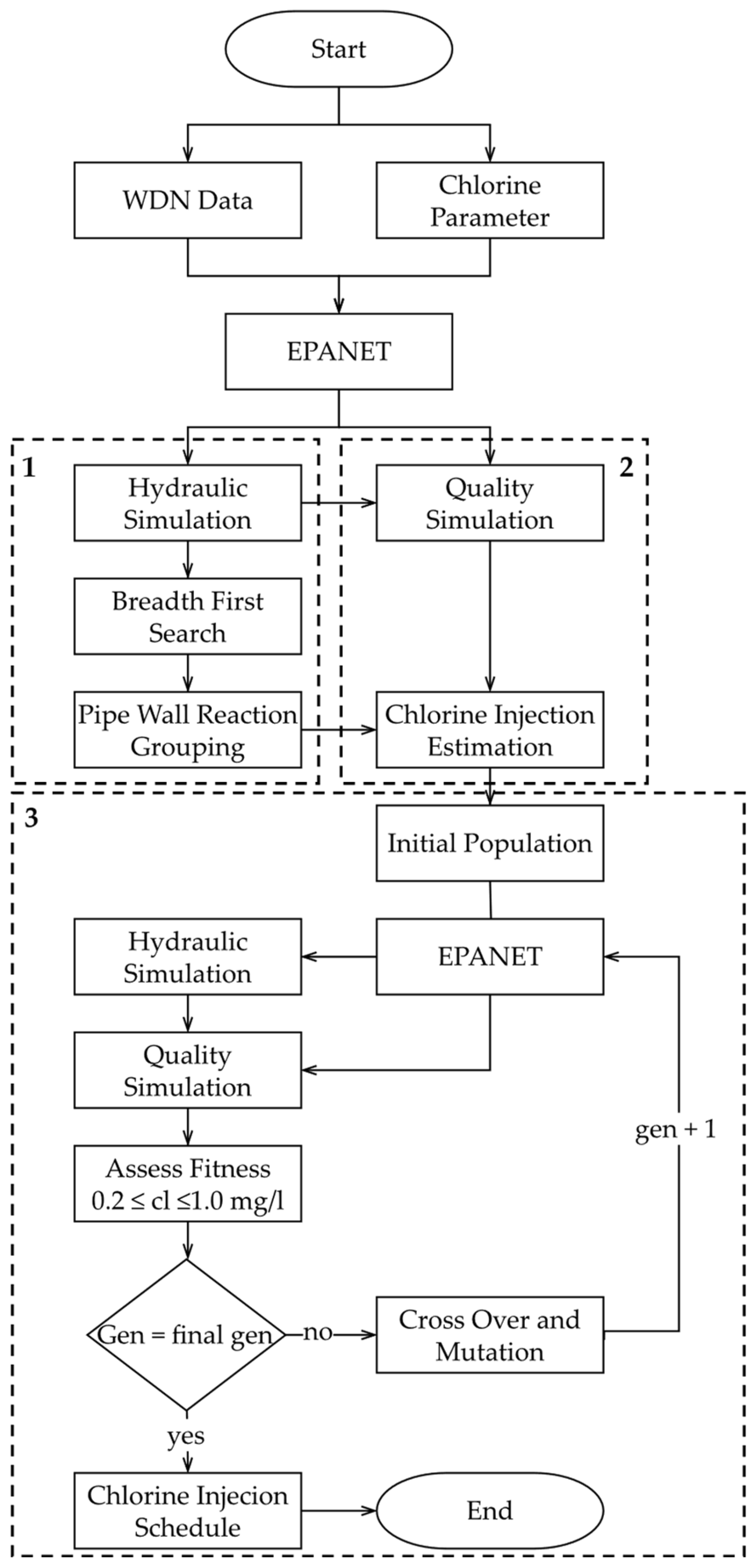
Figure 2.
Application network.
Figure 2.
Application network.
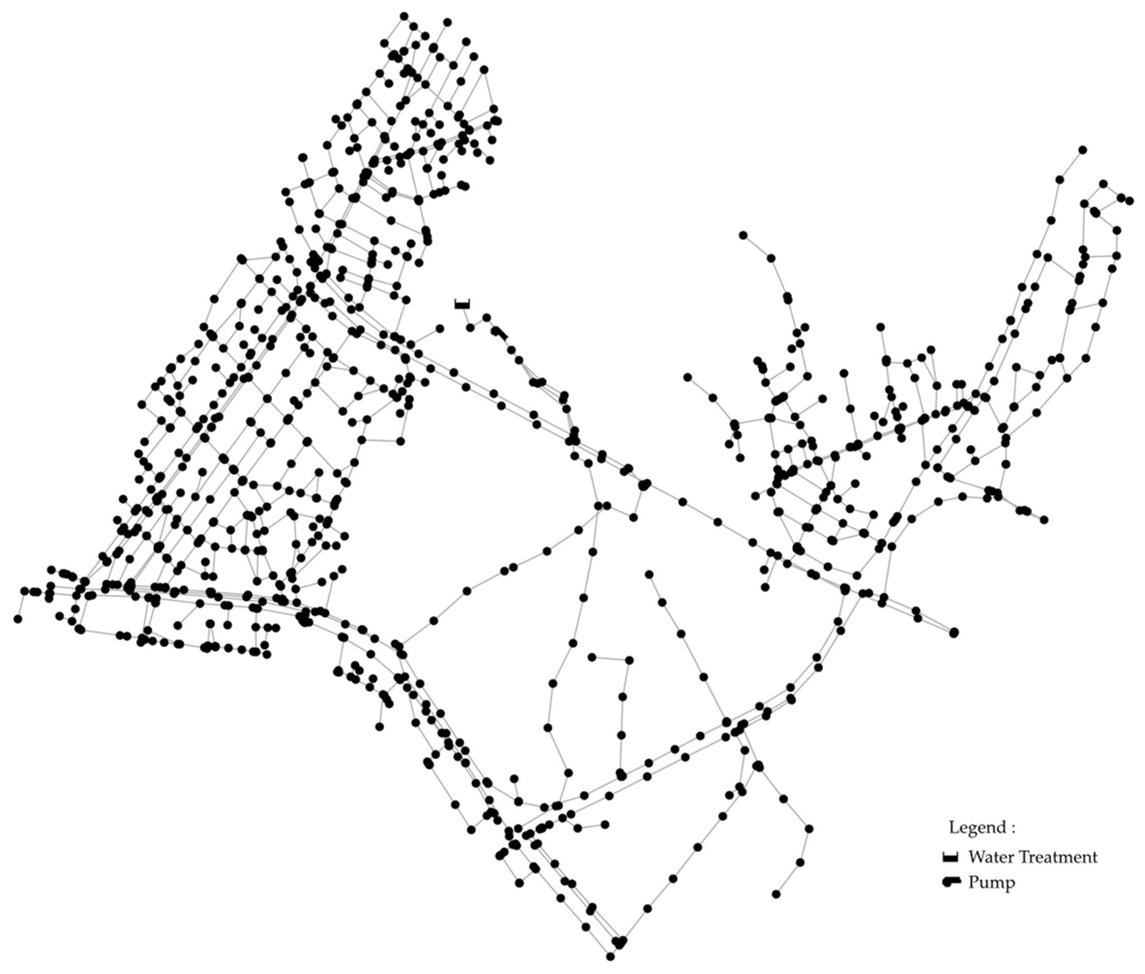
Figure 3.
Demand pattern and injection schedule interval of Scenario 2.
Figure 3.
Demand pattern and injection schedule interval of Scenario 2.
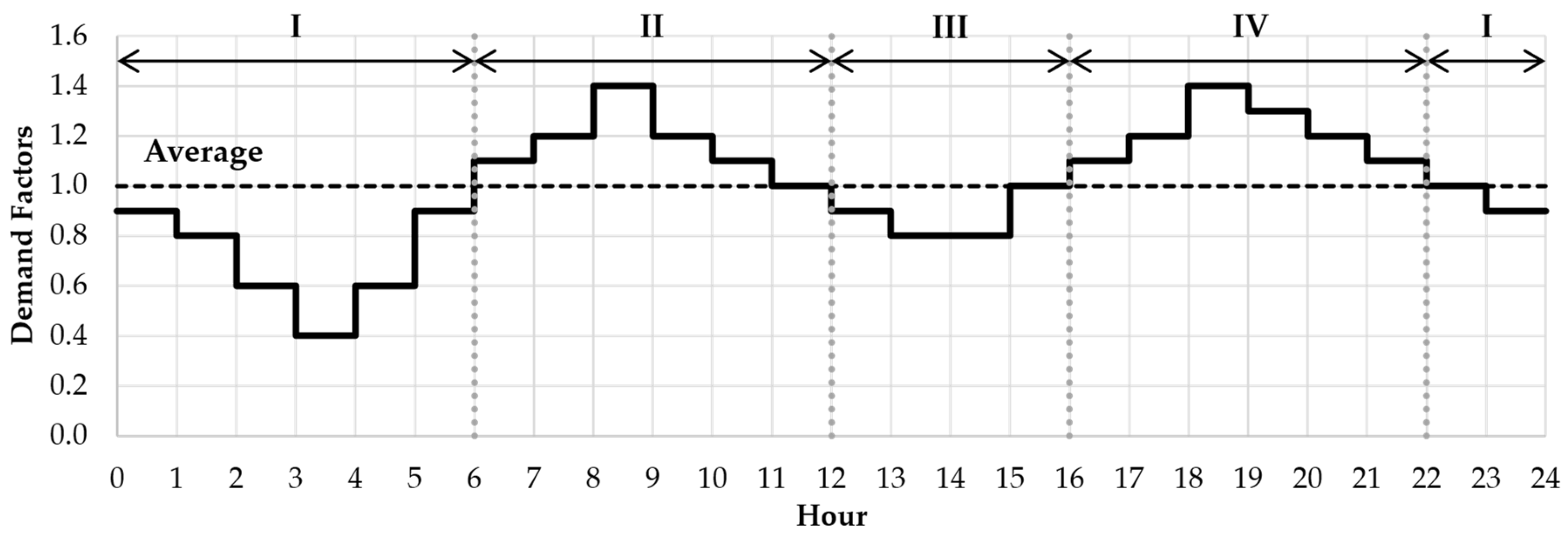
Figure 4.
Demonstration of BFS in a sample WDN.
Figure 4.
Demonstration of BFS in a sample WDN.
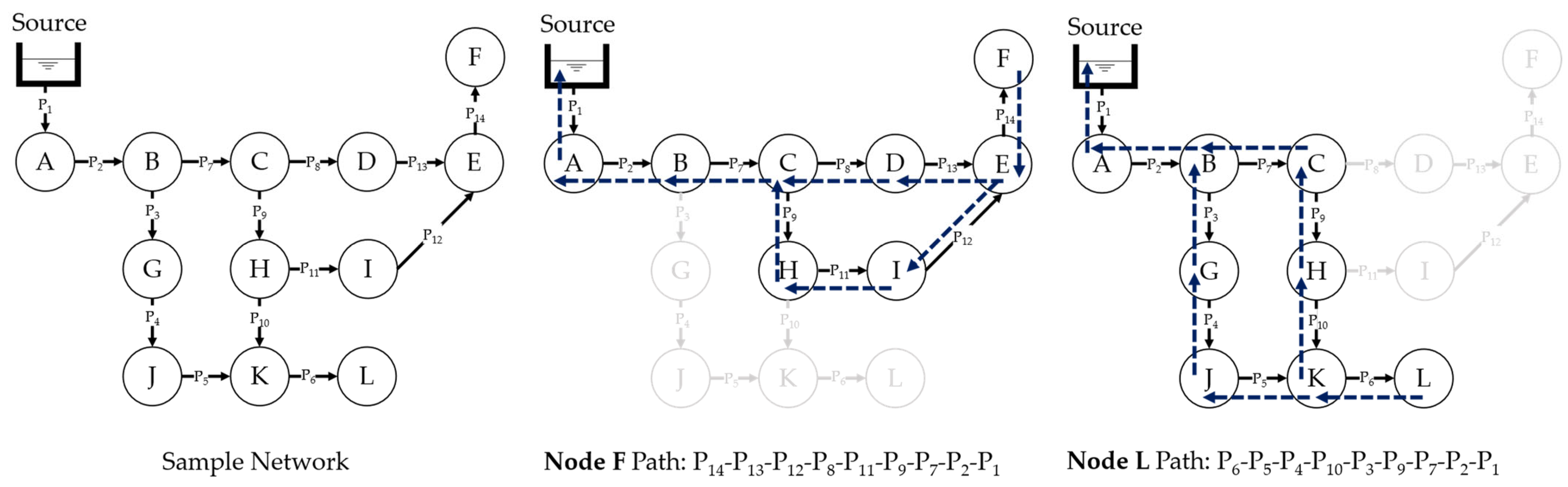
Figure 5.
Required chlorine injection estimation in a sample WDN: (a) required chlorine injection at hour 4; (b) required chlorine injection at hour 19.
Figure 5.
Required chlorine injection estimation in a sample WDN: (a) required chlorine injection at hour 4; (b) required chlorine injection at hour 19.
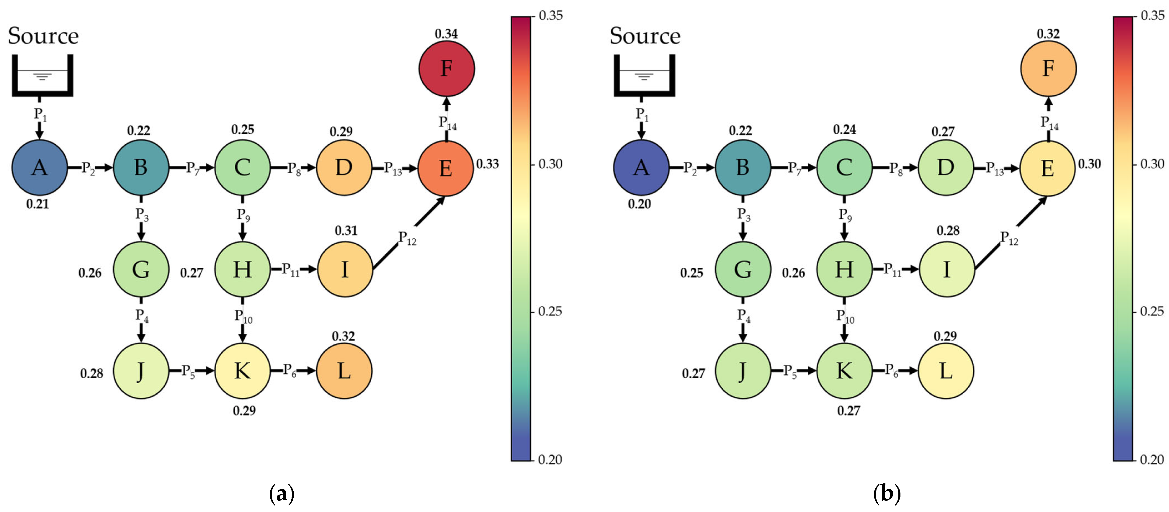
Figure 6.
Required source-injection chlorine concentration for each node at hours 4 and 19: (a) required chlorine injection at hour 4; (b) required chlorine injection at hour 19.
Figure 6.
Required source-injection chlorine concentration for each node at hours 4 and 19: (a) required chlorine injection at hour 4; (b) required chlorine injection at hour 19.
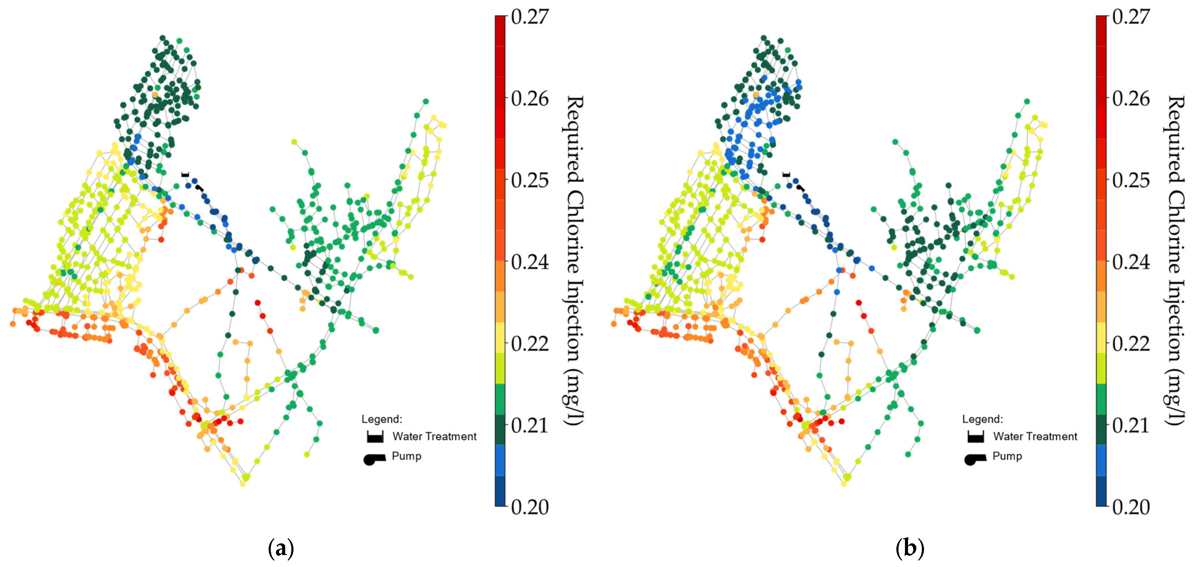
Figure 7.
Chlorine injection assessment: minimum, average, and maximum percentage of error (average value): (a) kb = 0.1056 day−1; (b) kb = 0.1872 day−1; (c) kb = 0.576 day−1.
Figure 7.
Chlorine injection assessment: minimum, average, and maximum percentage of error (average value): (a) kb = 0.1056 day−1; (b) kb = 0.1872 day−1; (c) kb = 0.576 day−1.
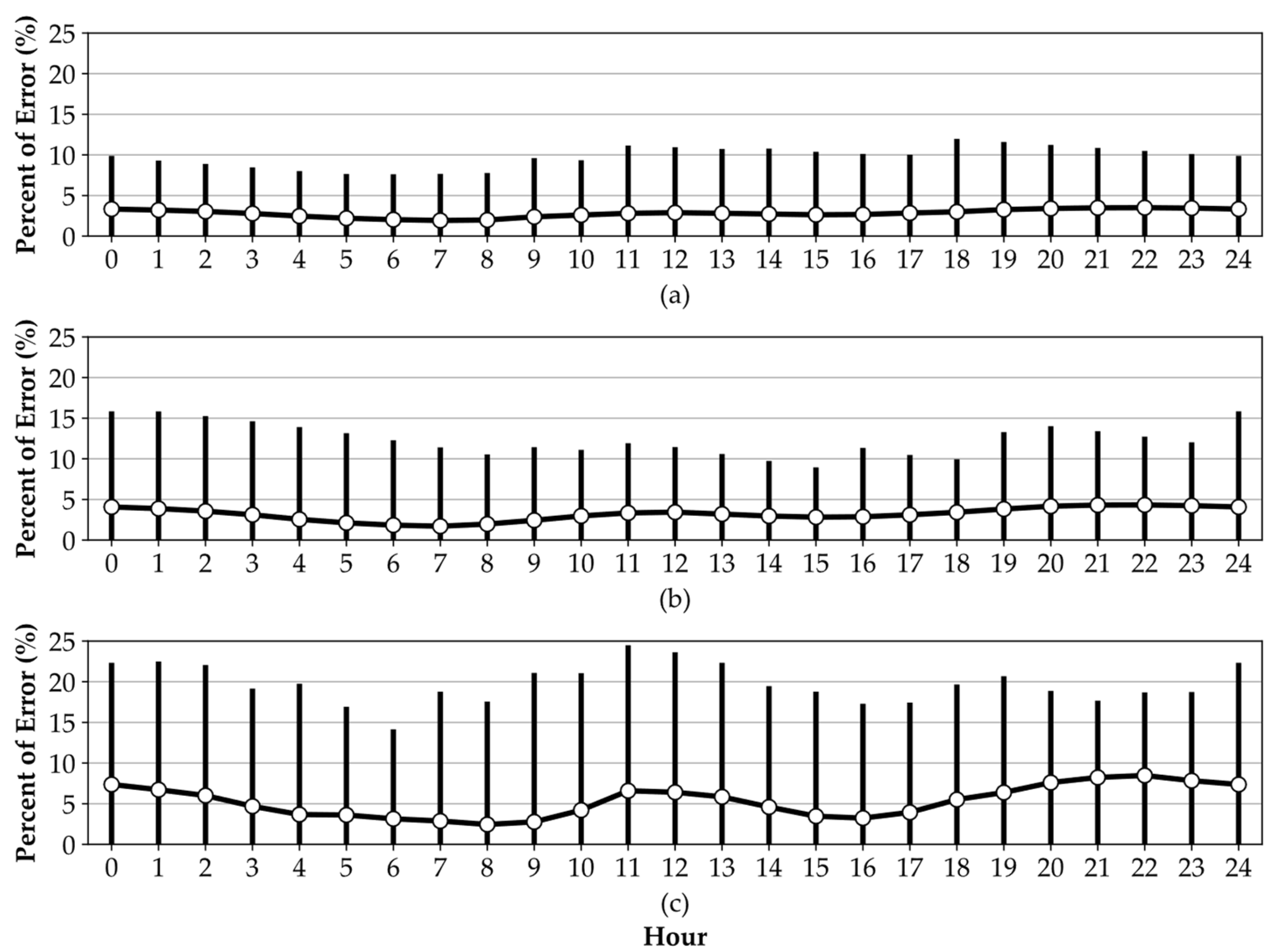
Figure 8.
Potential source-injection chlorine ranges for two injection scenarios: (a) single injection range; (b) 4-interval injection range.
Figure 8.
Potential source-injection chlorine ranges for two injection scenarios: (a) single injection range; (b) 4-interval injection range.
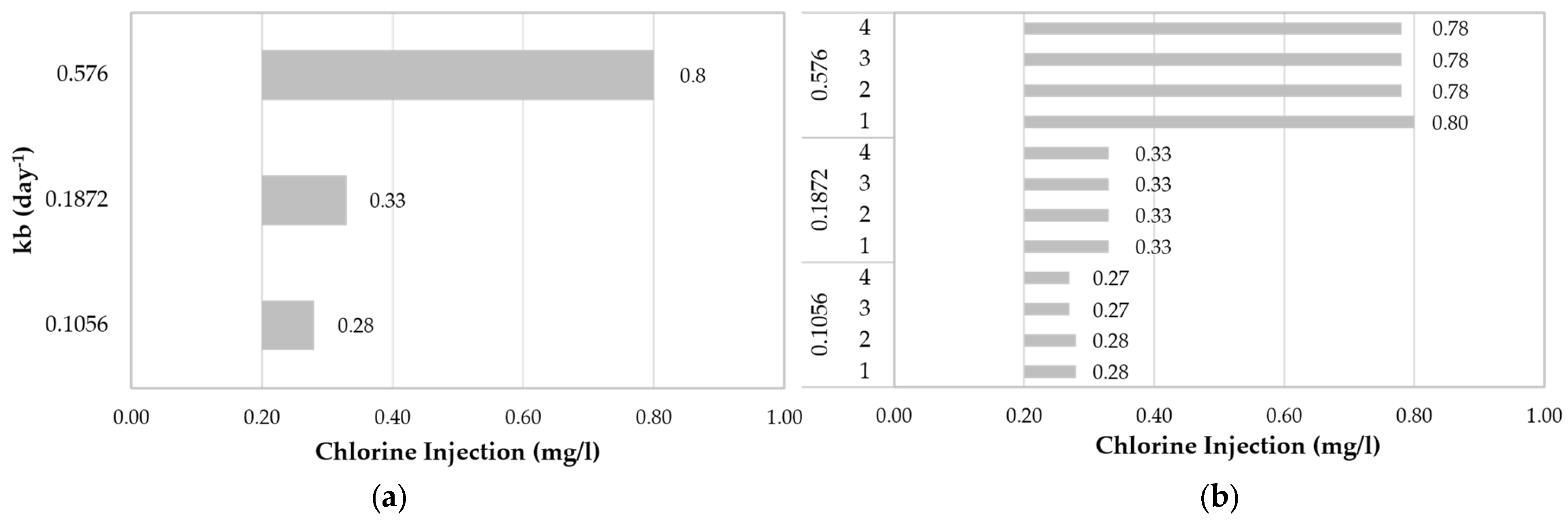
Figure 9.
Comparison of chlorine injection schedules at the source for two scenarios: (a) kb = 0.1056 day−1; (b) kb = 0.1872 day−1; (c) kb = 0.576 day−1.
Figure 9.
Comparison of chlorine injection schedules at the source for two scenarios: (a) kb = 0.1056 day−1; (b) kb = 0.1872 day−1; (c) kb = 0.576 day−1.
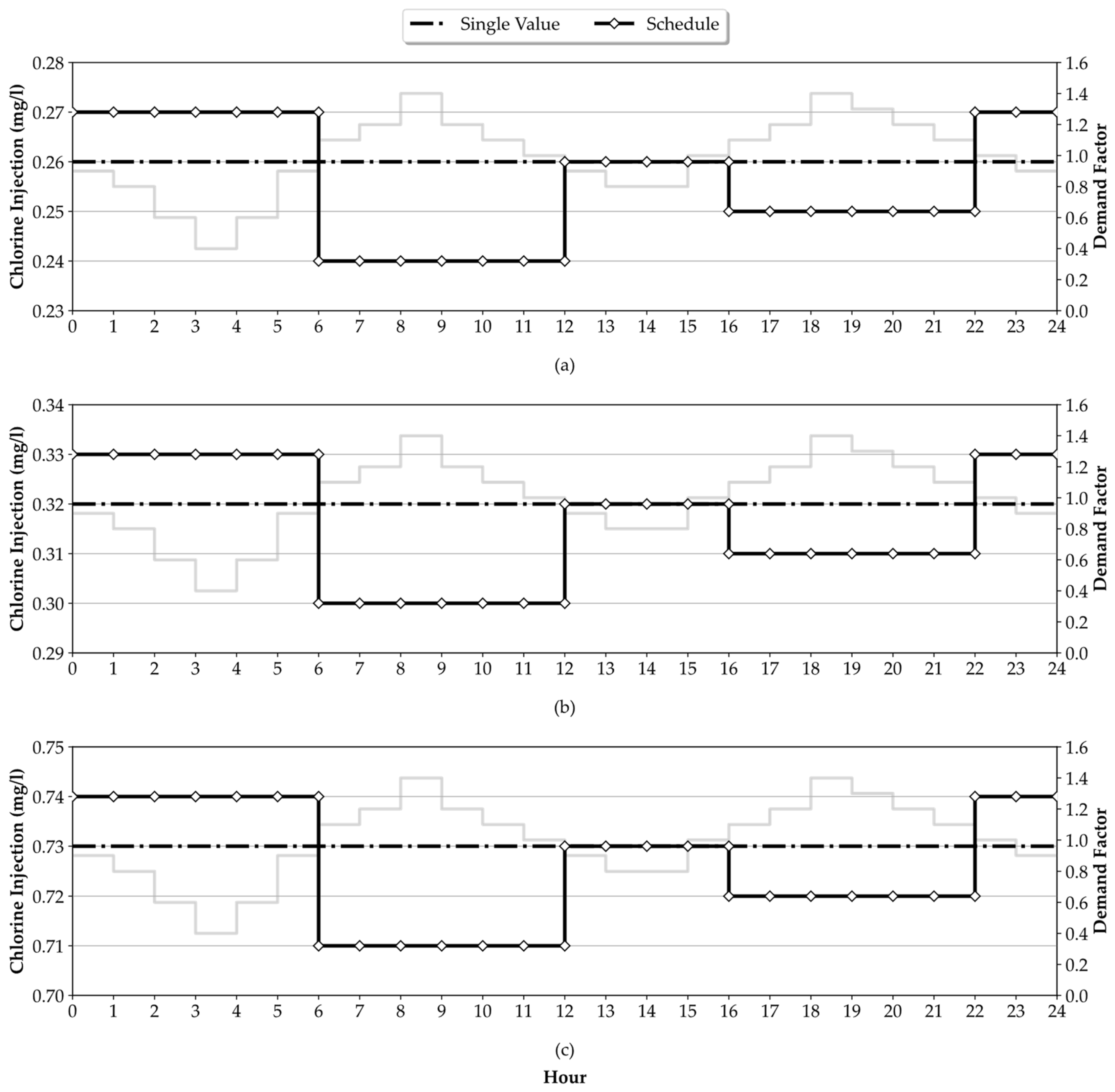
Figure 10.
System-wide temporal variation in residual chlorine concentration: (a) Scenario 1—kb = 0.1056 day−1; (b) Scenario 2—kb = 0.1056 day−1; (c) Scenario 1—kb = 0.1872 day−1; (d) Scenario 2—kb = 0.1872 day−1; (e) Scenario 1—kb = 0.576 day−1; (f) Scenario 2—kb = 0.576 day−1.
Figure 10.
System-wide temporal variation in residual chlorine concentration: (a) Scenario 1—kb = 0.1056 day−1; (b) Scenario 2—kb = 0.1056 day−1; (c) Scenario 1—kb = 0.1872 day−1; (d) Scenario 2—kb = 0.1872 day−1; (e) Scenario 1—kb = 0.576 day−1; (f) Scenario 2—kb = 0.576 day−1.
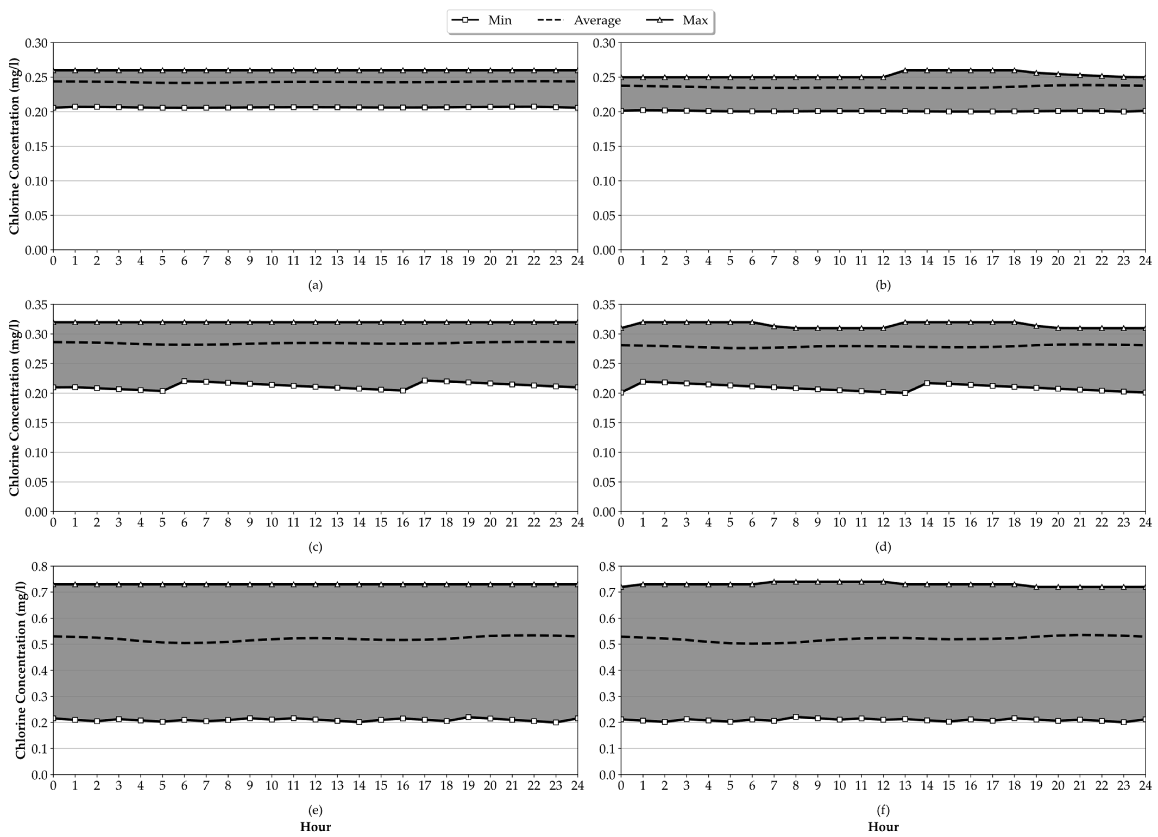
Figure 11.
Average nodal chlorine concentration for kb = 0.1056 day−1: (a) Scenario 1; (b) Scenario 2.
Figure 11.
Average nodal chlorine concentration for kb = 0.1056 day−1: (a) Scenario 1; (b) Scenario 2.
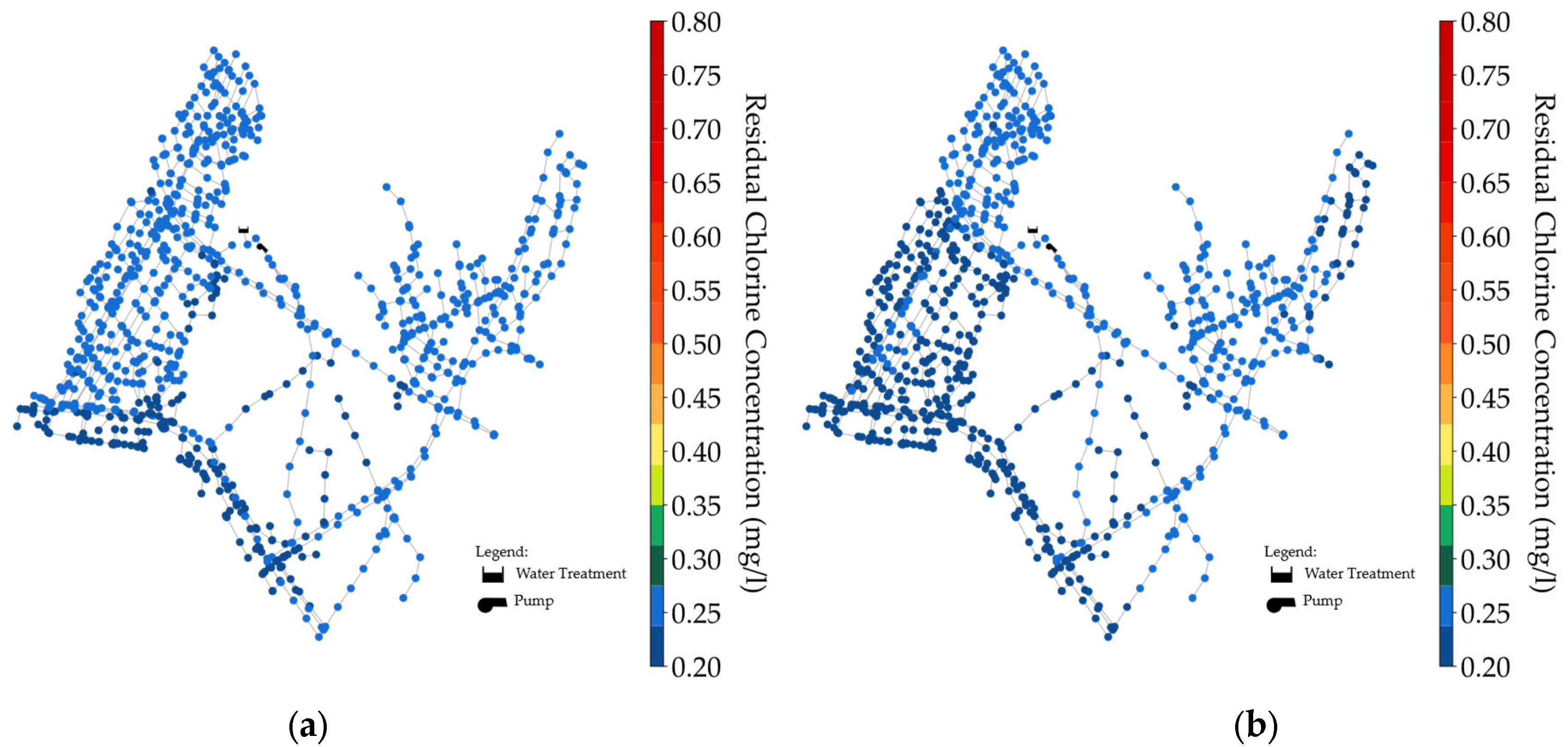
Figure 12.
Average nodal chlorine concentration for kb = 0.1872 day−1: (a) Scenario 1; (b) Scenario 2.
Figure 12.
Average nodal chlorine concentration for kb = 0.1872 day−1: (a) Scenario 1; (b) Scenario 2.
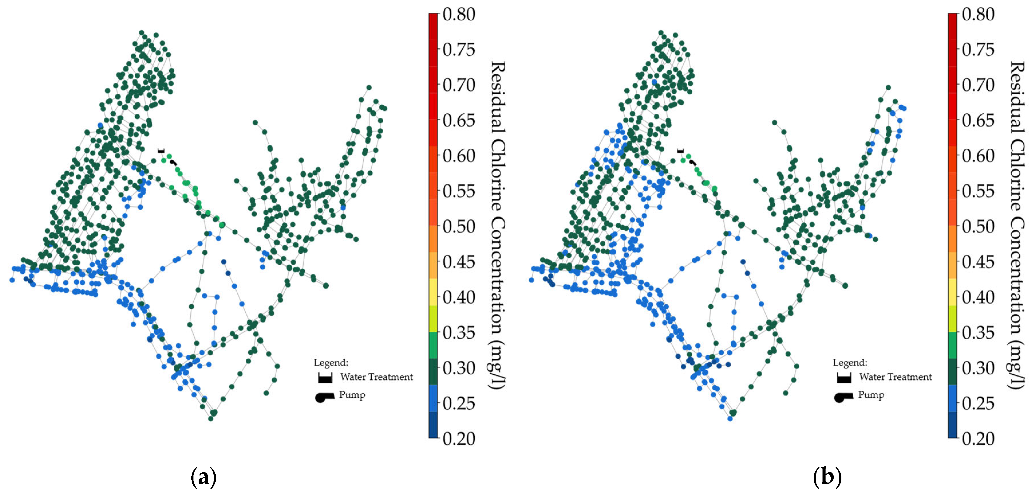
Figure 13.
Average nodal chlorine concentration for kb = 0.576 day−1: (a) Scenario 1; (b) Scenario 2.
Figure 13.
Average nodal chlorine concentration for kb = 0.576 day−1: (a) Scenario 1; (b) Scenario 2.
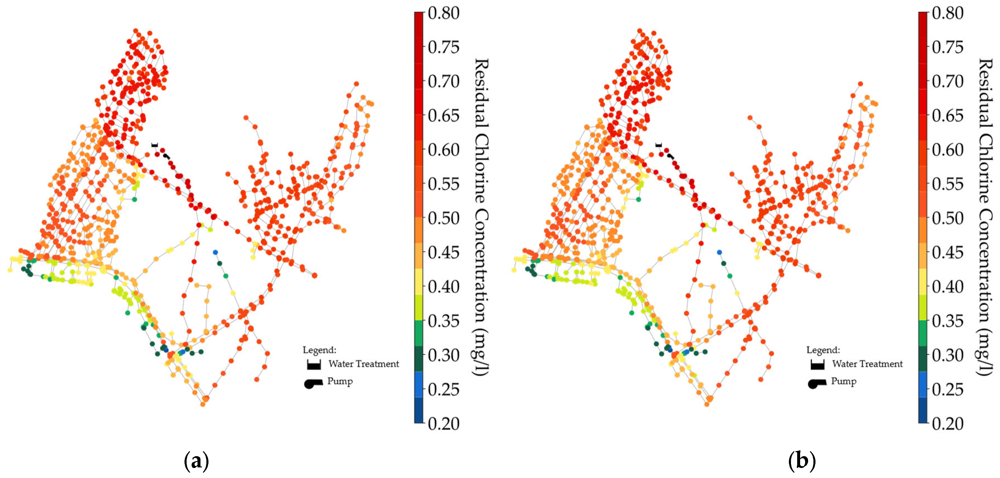
Table 1.
Chlorine parameter data.
Table 1.
Chlorine parameter data.
| Temp (°C) | (day−1) | (m2/s) | (m2/s) |
|---|---|---|---|
| 4.5 | 0.1056 | 1.55 × 10⁻⁶ | 6.74 × 10⁻¹⁰ |
| 18.0 | 0.1872 | 1.06 × 10⁻⁶ | 1.14 × 10⁻⁹ |
| 25.0 | 0.576 | 9.03 × 10⁻⁷ | 1.38 × 10⁻⁹ |
Table 2.
Chlorine injection scenarios.
Table 2.
Chlorine injection scenarios.
| Scenario | Operation Method | Number of Decision Variable | Interval Time Step (hour) |
|---|---|---|---|
| 1 | Single Injection | 1 | 24 |
| 2 | 4-Interval Injection | 4 | 8–6–4–6 |
Table 3.
Statistics of optimal results for two scenarios.
Table 3.
Statistics of optimal results for two scenarios.
| Statistics | kb = 0.1056 | kb = 0.1872 | kb = 0.576 | |||
|---|---|---|---|---|---|---|
| Sce.1 | Sce.2 | Sce.1 | Sce.2 | Sce.1 | Sce.2 | |
| Mean Concentration (mg/L) | 0.243 | 0.237 | 0.279 | 0.285 | 0.521 | 0.516 |
| Standard Deviation Concentration (mg/L) * | 0.044 | 0.038 | 0.086 | 0.081 | 0.332 | 0.328 |
| Minimum Concentration (mg/L) | 0.206 | 0.200 | 0.204 | 0.200 | 0.200 | 0.200 |
| Maximum Concentration (mg/L) | 0.260 | 0.270 | 0.320 | 0.330 | 0.730 | 0.740 |
| Dosage Input (kg/day) [A] | 92.7 | 90.5 | 114.1 | 111.9 | 260.3 | 258.1 |
| Dosage Output (kg/day) [B] | 87.0 | 84.8 | 102.0 | 99.9 | 188.4 | 186.7 |
| Dosage Decay (kg/day) [A-B-C] | 8.0 | 7.9 | 14.8 | 14.6 | 77.2 | 76.6 |
| Dosage Storage Change (kg/day) [C] | −2.26 | −2.21 | −2.68 | −2.63 | −5.20 | −5.15 |
|
Disclaimer/Publisher’s Note: The statements, opinions and data contained in all publications are solely those of the individual author(s) and contributor(s) and not of MDPI and/or the editor(s). MDPI and/or the editor(s) disclaim responsibility for any injury to people or property resulting from any ideas, methods, instructions or products referred to in the content. |