Prediction of Soil Erosion Using 3D Point Scans and Acoustic Emissions
[ad_1]
Author Contributions
Conceptualization, J.W. and M.F.A.D.; methodology, J.W. and M.F.A.D.; software, J.W. and M.F.A.D.; validation, J.W. and M.F.A.D.; formal analysis, J.W. and M.F.A.D.; investigation, J.W. and M.F.A.D.; resources, J.W. and M.F.A.D.; data curation, J.W. and M.F.A.D.; writing—original draft preparation, J.W. and M.F.A.D.; writing—review and editing, J.W. and M.F.A.D.; visualization, J.W. and M.F.A.D.; supervision, J.W. and M.F.A.D.; project administration, J.W. and M.F.A.D. All authors have read and agreed to the published version of the manuscript.
Figure 1.
Schematic of the erosion test flume.
Figure 1.
Schematic of the erosion test flume.
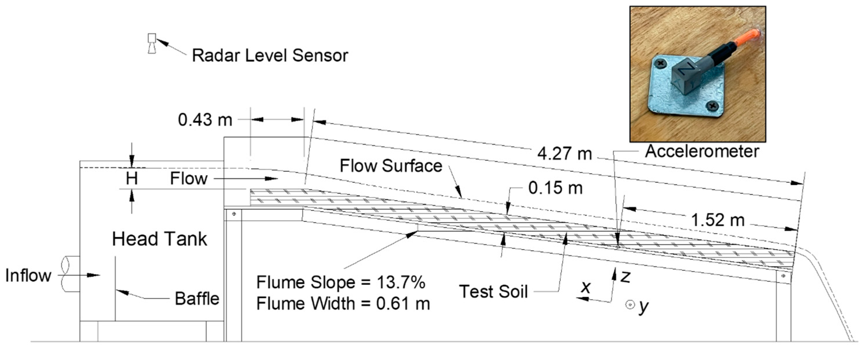
Figure 2.
Raw discharge data and acceleration data in the three directions with respect to relative time.
Figure 2.
Raw discharge data and acceleration data in the three directions with respect to relative time.
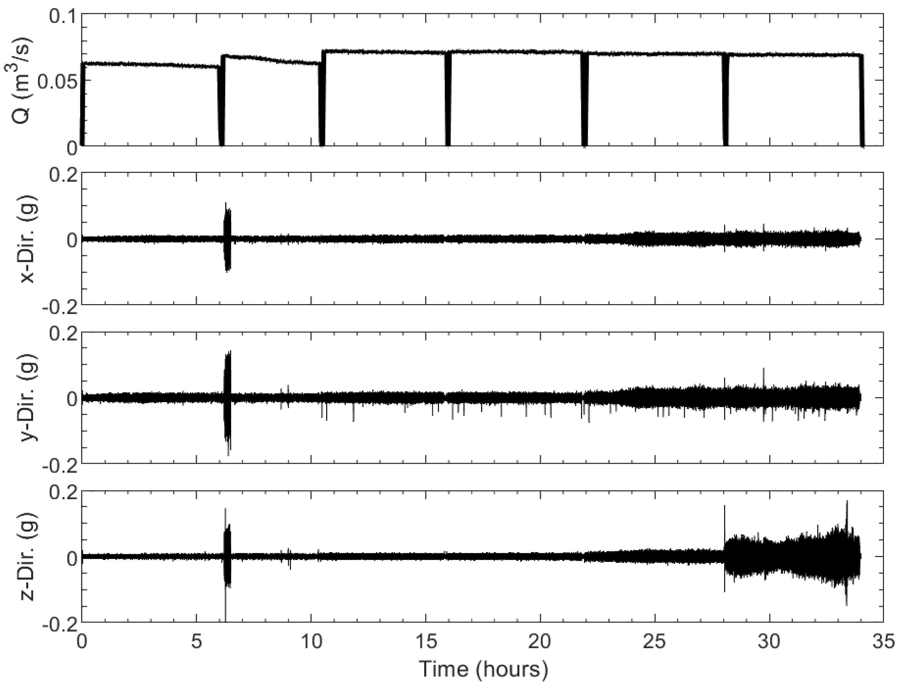
Figure 3.
(a) Campbell Scientific CS475A water radar sensor used for autonomous discharge measurement. (b) Gravity head tank that provided the water discharge for the test. (c) Erosion of the soil at the inlet of the test flume.
Figure 3.
(a) Campbell Scientific CS475A water radar sensor used for autonomous discharge measurement. (b) Gravity head tank that provided the water discharge for the test. (c) Erosion of the soil at the inlet of the test flume.
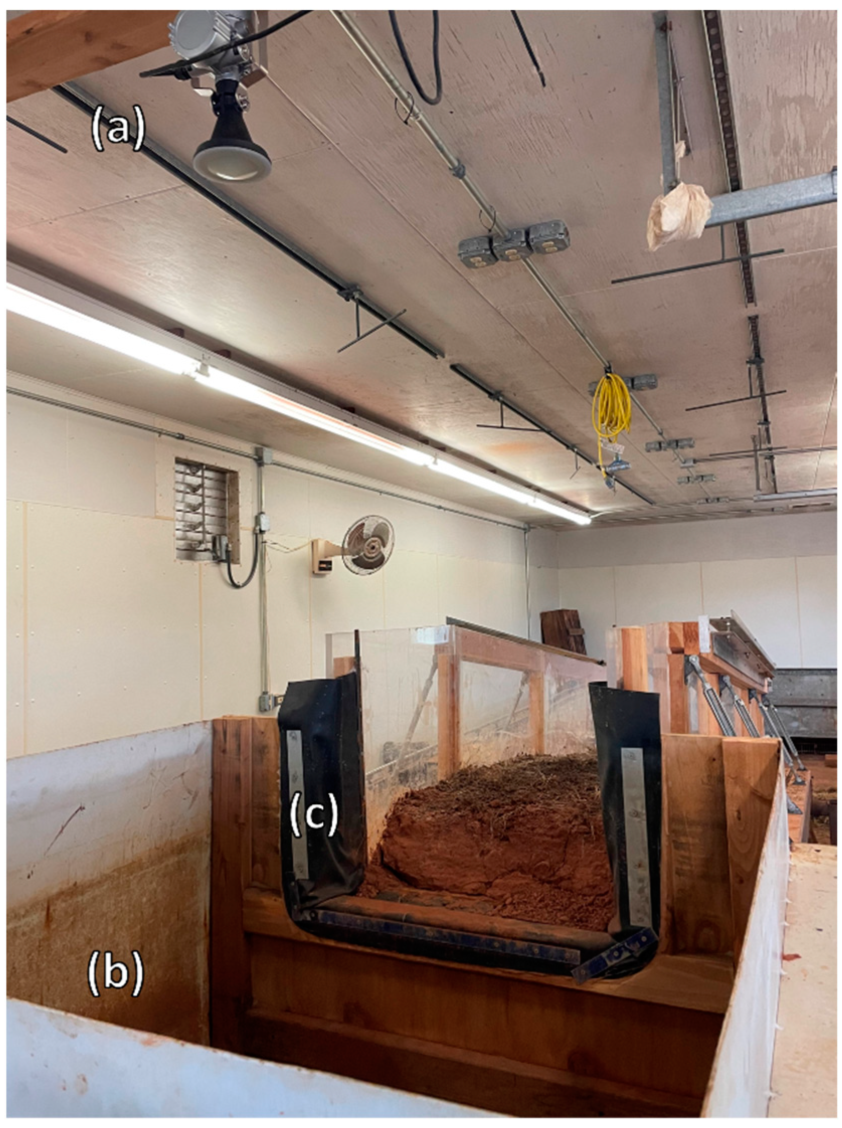
Figure 4.
3D point cloud scans depicting the progression of soil erosion during testing. Note that the orange color represents high spots, and the dark blue represents voids (i.e., erosion).
Figure 4.
3D point cloud scans depicting the progression of soil erosion during testing. Note that the orange color represents high spots, and the dark blue represents voids (i.e., erosion).
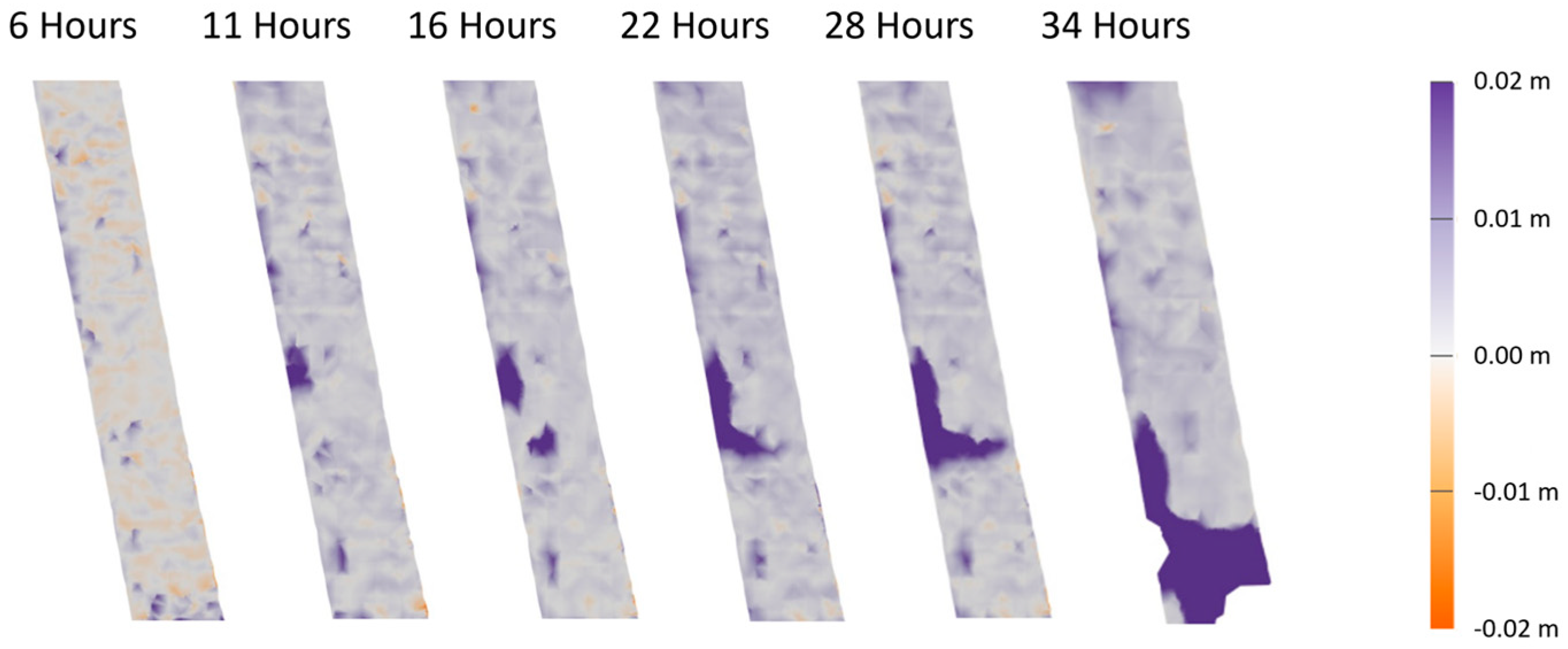
Figure 5.
Quantified soil erosion values throughout testing with a trendline (dashed line) showing the linear relationship between erosion and time before the failure point.
Figure 5.
Quantified soil erosion values throughout testing with a trendline (dashed line) showing the linear relationship between erosion and time before the failure point.
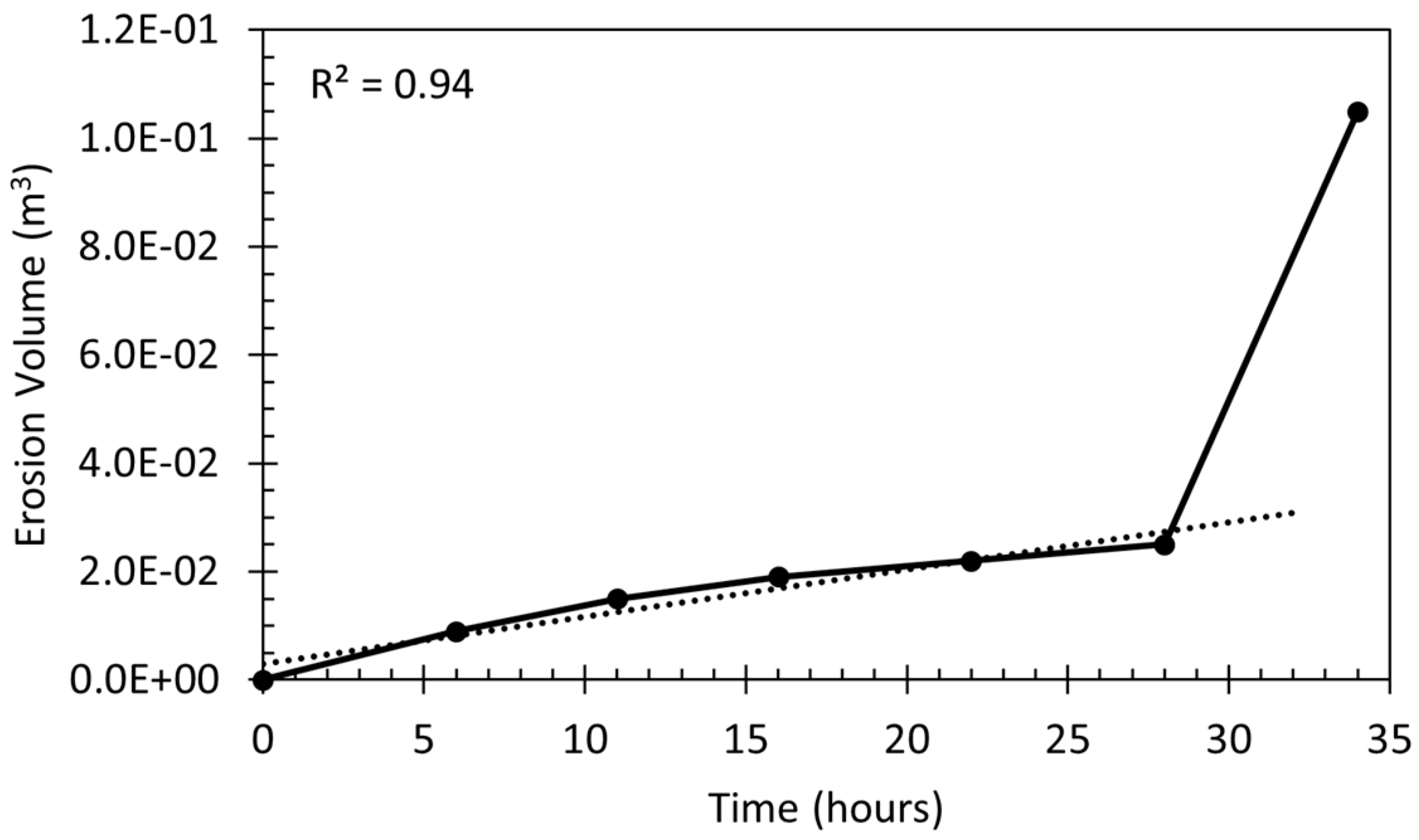
Figure 6.
(a) Final scan of the test flume showing the eroded soil. This erosion event is referenced as the failure point of the test. (b) Zoomed in region showing the exposed accelerometer.
Figure 6.
(a) Final scan of the test flume showing the eroded soil. This erosion event is referenced as the failure point of the test. (b) Zoomed in region showing the exposed accelerometer.
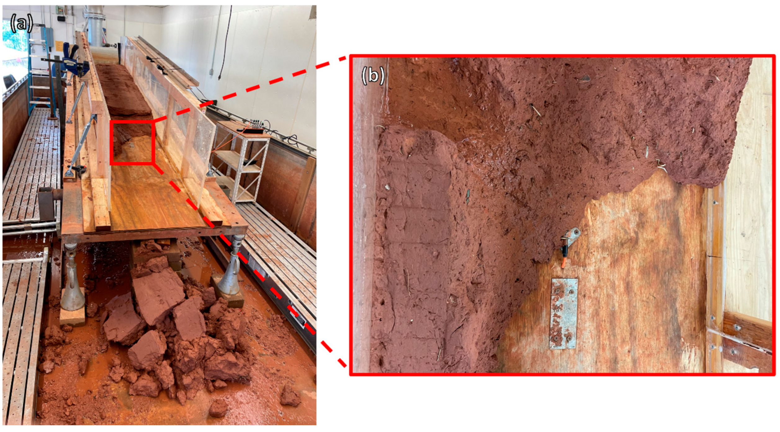
Figure 7.
20 s acceleration data in all three directions for the range of sampling rates.
Figure 7.
20 s acceleration data in all three directions for the range of sampling rates.
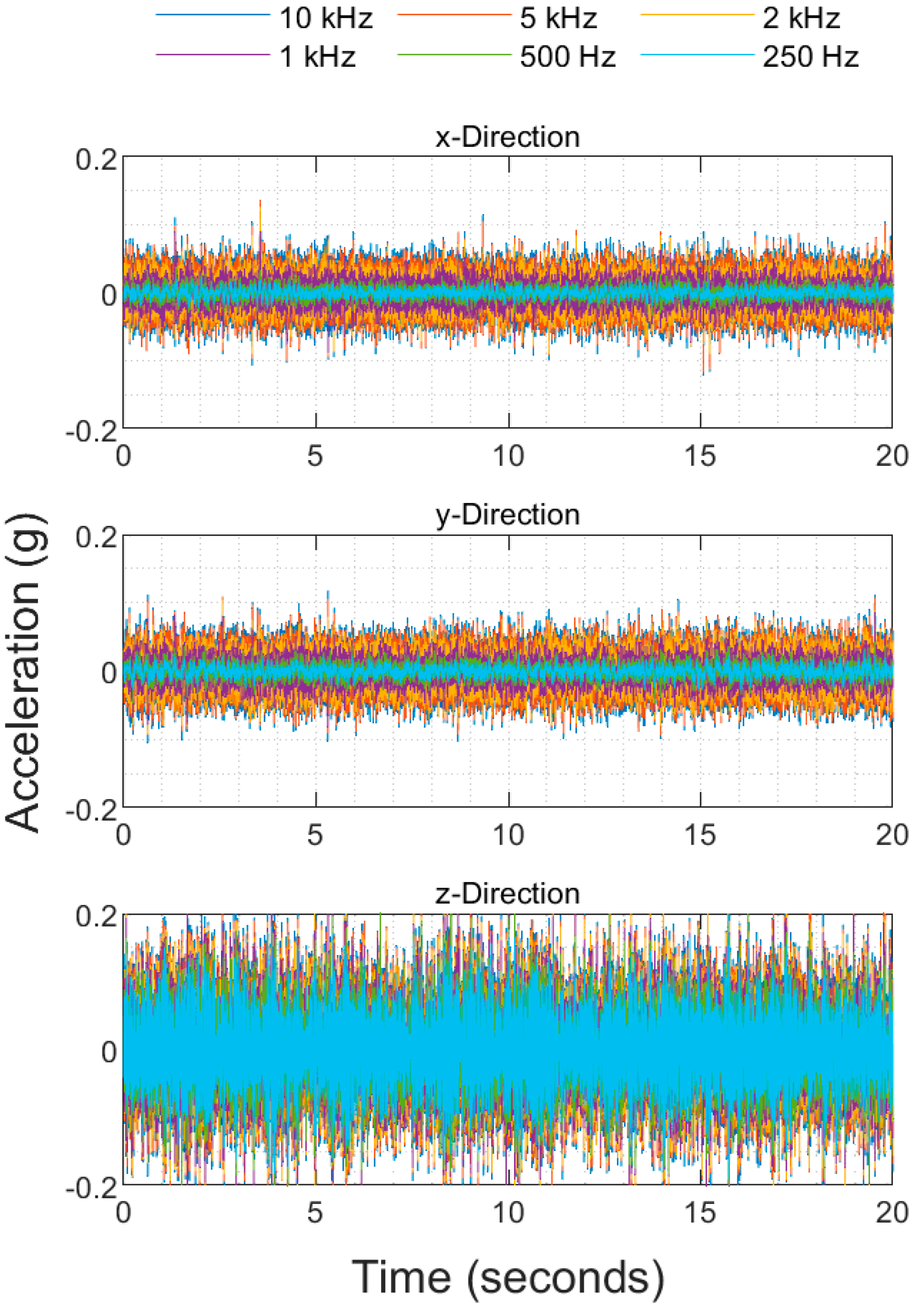
Figure 8.
PSD response at the 1 h time interval for all three directions with different sampling rates.
Figure 8.
PSD response at the 1 h time interval for all three directions with different sampling rates.
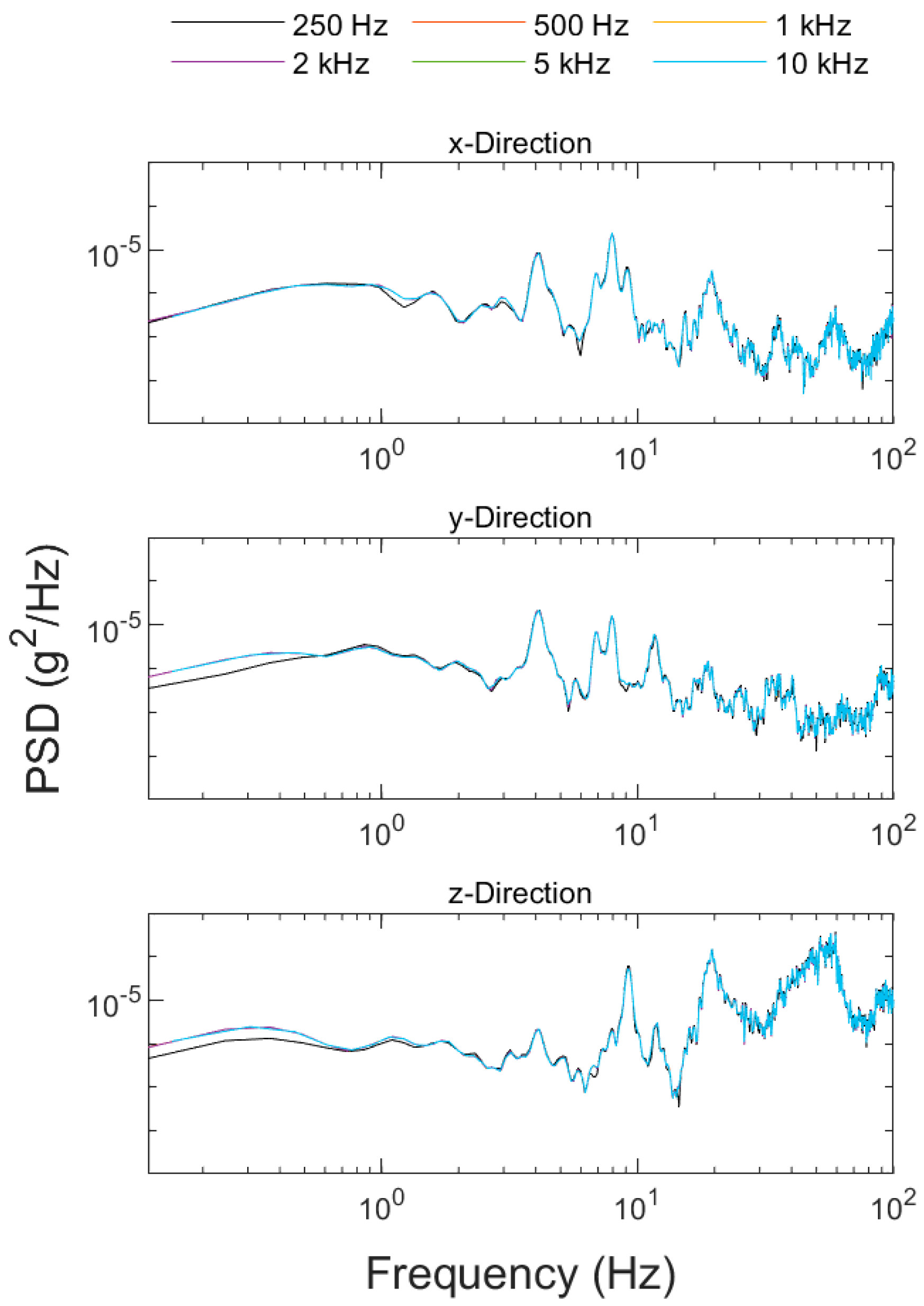
Figure 9.
Acceleration data for the seven time intervals in the x-, y-, and z-directions.
Figure 9.
Acceleration data for the seven time intervals in the x-, y-, and z-directions.
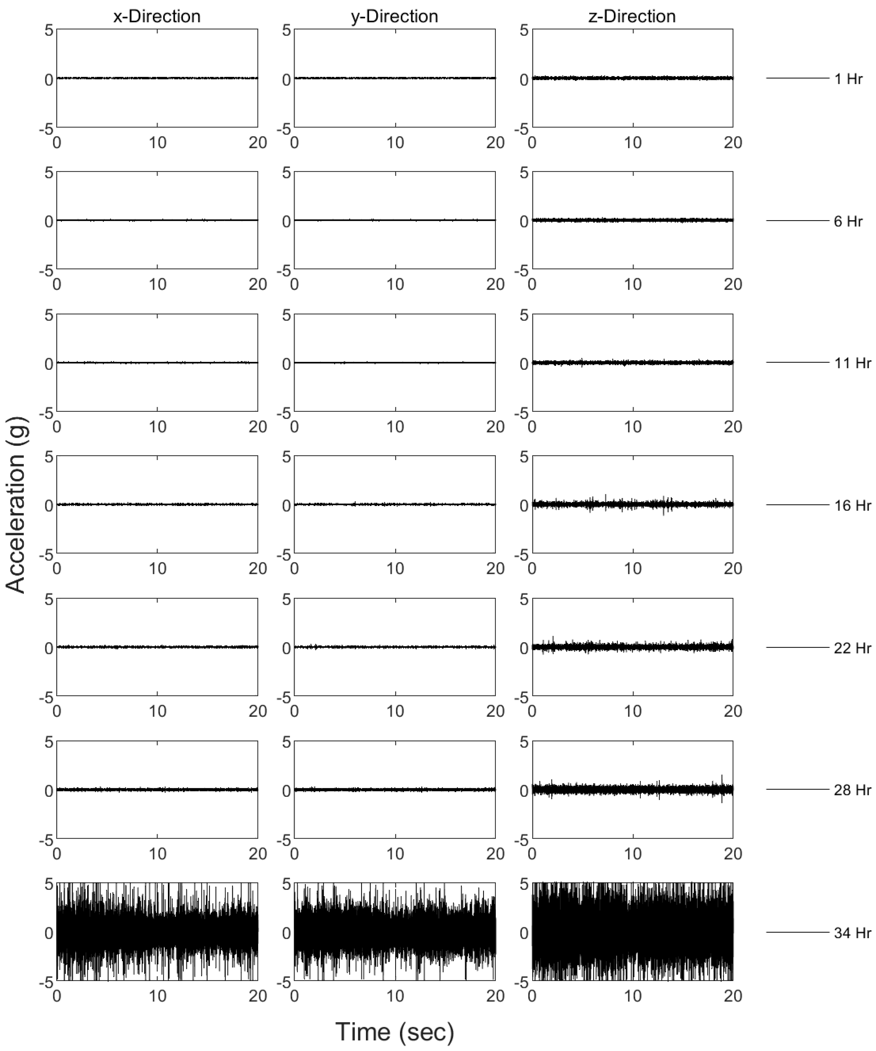
Figure 10.
PSD versus frequency analysis for the x-, y-, and z-directions.
Figure 10.
PSD versus frequency analysis for the x-, y-, and z-directions.
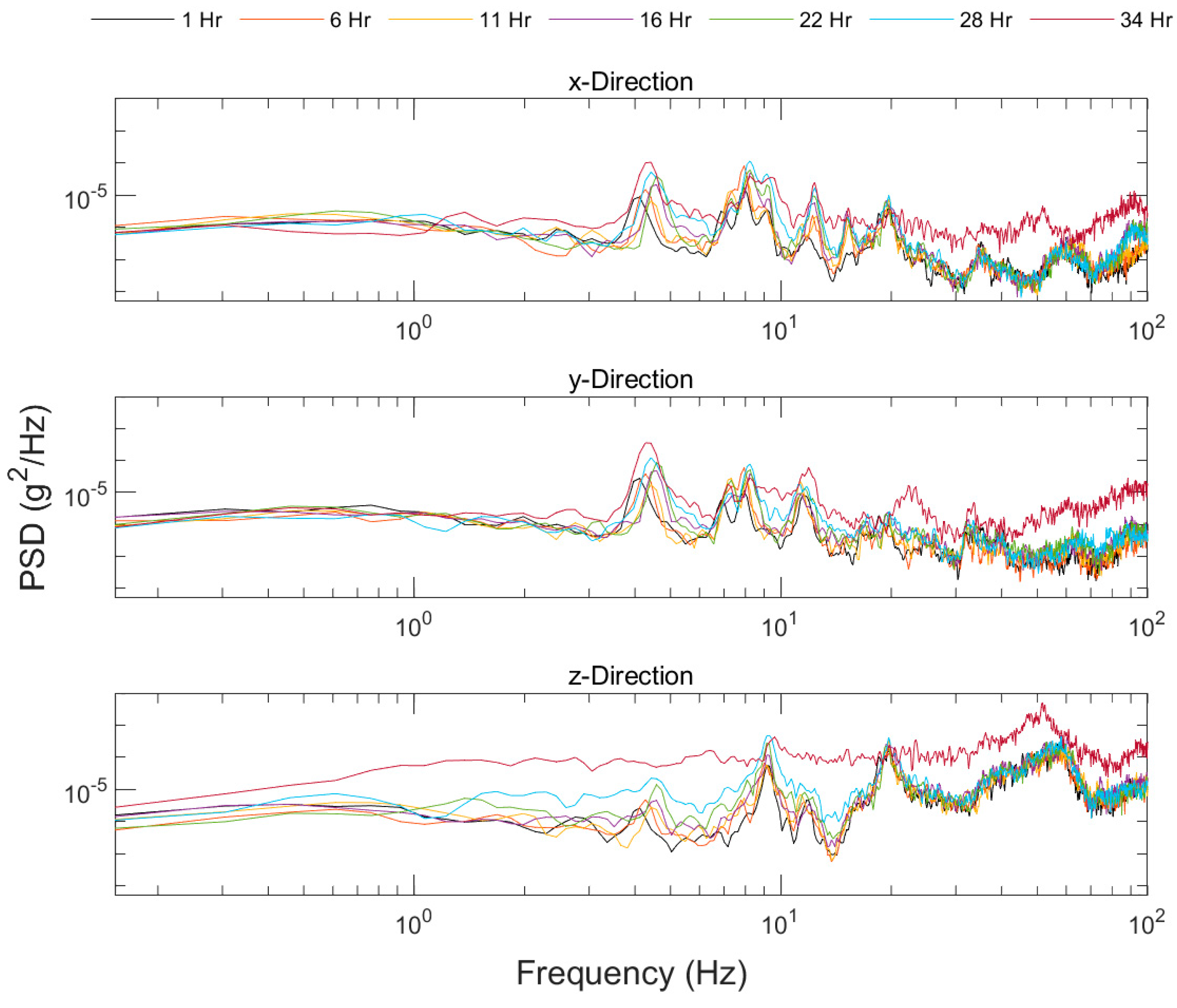
Figure 11.
Magnified pre-erosion PSD versus frequency data for the x-, y-, and z-directions.
Figure 11.
Magnified pre-erosion PSD versus frequency data for the x-, y-, and z-directions.

Figure 12.
Averaged and normalized PSD power for each direction from 0 to 100 Hz.
Figure 12.
Averaged and normalized PSD power for each direction from 0 to 100 Hz.
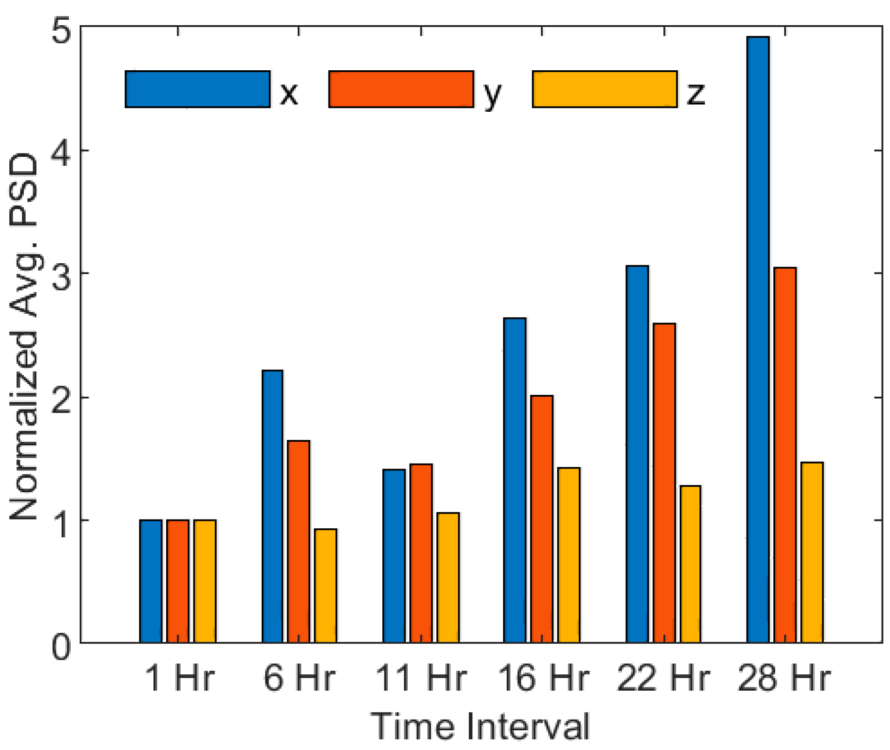
Figure 13.
PSD power amplitudes versus time for all three axes. The pre-erosion amplitudes follow a linear trend as indicated by the dotted trendlines and their respective coefficients of determination.
Figure 13.
PSD power amplitudes versus time for all three axes. The pre-erosion amplitudes follow a linear trend as indicated by the dotted trendlines and their respective coefficients of determination.

Figure 14.
PSD power and erosion of the test with respect to time.
Figure 14.
PSD power and erosion of the test with respect to time.
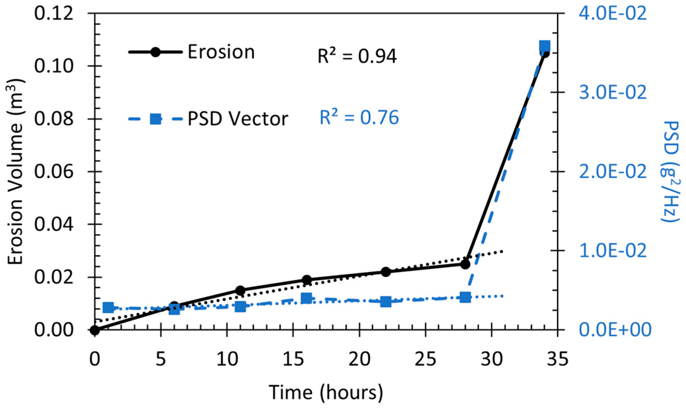
Figure 15.
PSD power spectra versus erosion volume values and their resulting linear relationship.
Figure 15.
PSD power spectra versus erosion volume values and their resulting linear relationship.
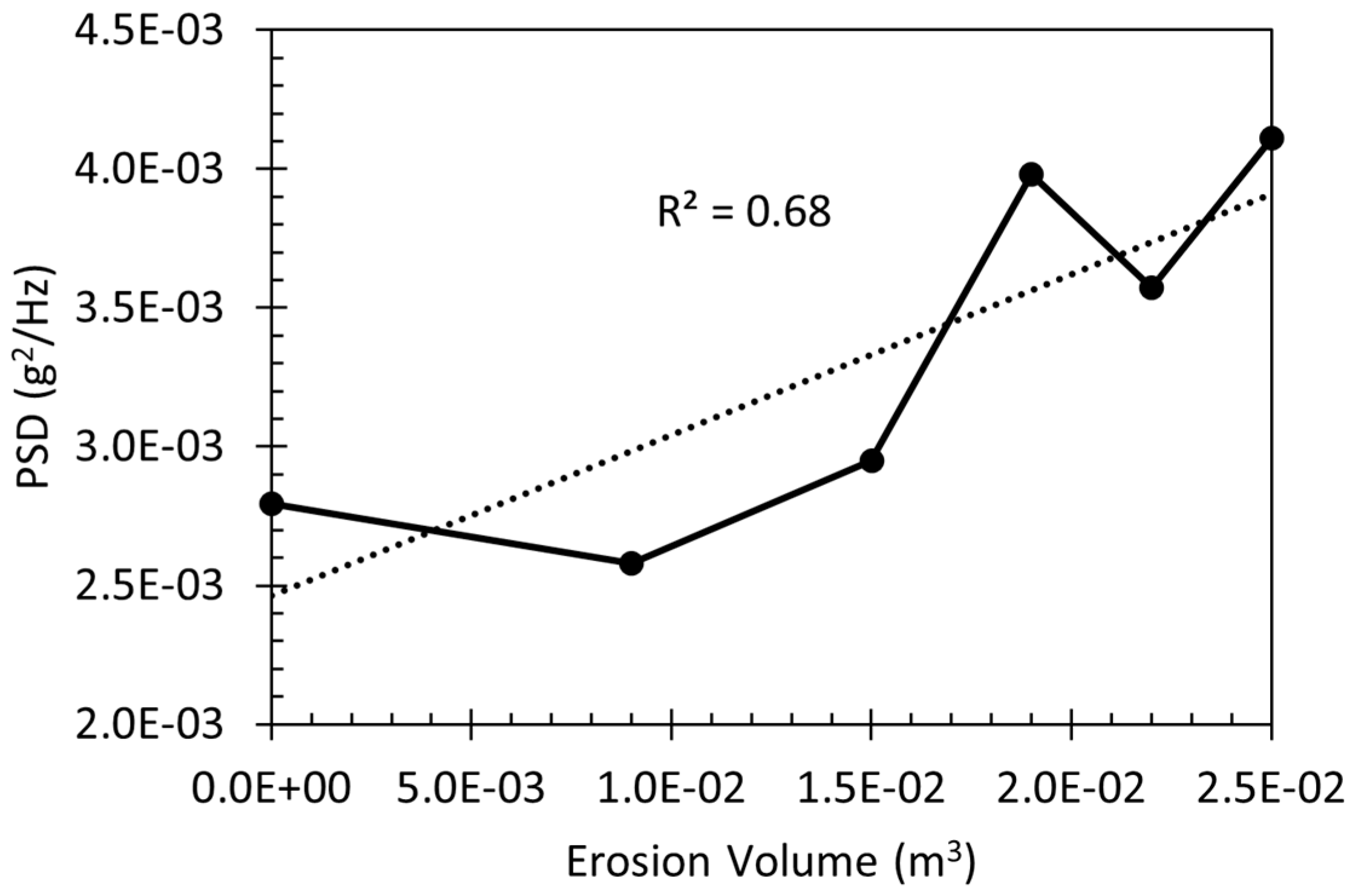
Table 1.
Percent difference of the average PSD power for each sampling rate compared to the original 10 kHz sampling rate at the 1 h time interval.
Table 1.
Percent difference of the average PSD power for each sampling rate compared to the original 10 kHz sampling rate at the 1 h time interval.
| Sampling | x-Axis | y-Axis | z-Axis |
|---|---|---|---|
| Rate | % Diff. | % Diff. | % Diff. |
| 250 Hz | 0.08% | 0.08% | 0.07% |
| 500 Hz | 0.05% | 0.04% | 0.04% |
| 1 kHz | 0.02% | 0.02% | 0.07% |
| 2 kHz | 0.01% | 0.02% | 0.04% |
| 5 kHz | 0.00% | 0.00% | −0.01% |
| 10 kHz | – | – | – |
Table 2.
Percent difference of the average PSD power compared to the original sampling rate during the 34 h time interval.
Table 2.
Percent difference of the average PSD power compared to the original sampling rate during the 34 h time interval.
| Sampling | x-Axis | y-Axis | z-Axis |
|---|---|---|---|
| Rate | % Diff. | % Diff. | % Diff. |
| 1 kHz | 0.02% | 0.02% | 0.08% |
| 5 kHz | −0.01% | −0.01% | −0.01% |
| 10 kHz | – | – | – |
[ad_2]