Automation and Robots for Disaster Response

Species-Level Classification of Peatland Vegetation Using Ultra-High-Resolution UAV Imagery

By inergency On Mar 13, 2024

[ad_1]

Figure 1.
UAV surveying at Auchencorth Moss. Shown in (a) is the custom-built Tarot T680 Pro (Wenzhou Tarot Aviation Technology Co., Wenzhou, China) and mounted Parrot Sequoia camera positioned over a spectral calibration panel (photo credit: G. Simpson). Shown on the right are photographs taken with the Mavic 2 Pro (SZ DJI Technology Co., Ltd., Shenzhen, China): (b) is an aerial photograph of the survey area; and (c) shows one of the individual images acquired during the RGB survey, which highlights the strong spatial heterogeneity of the site.

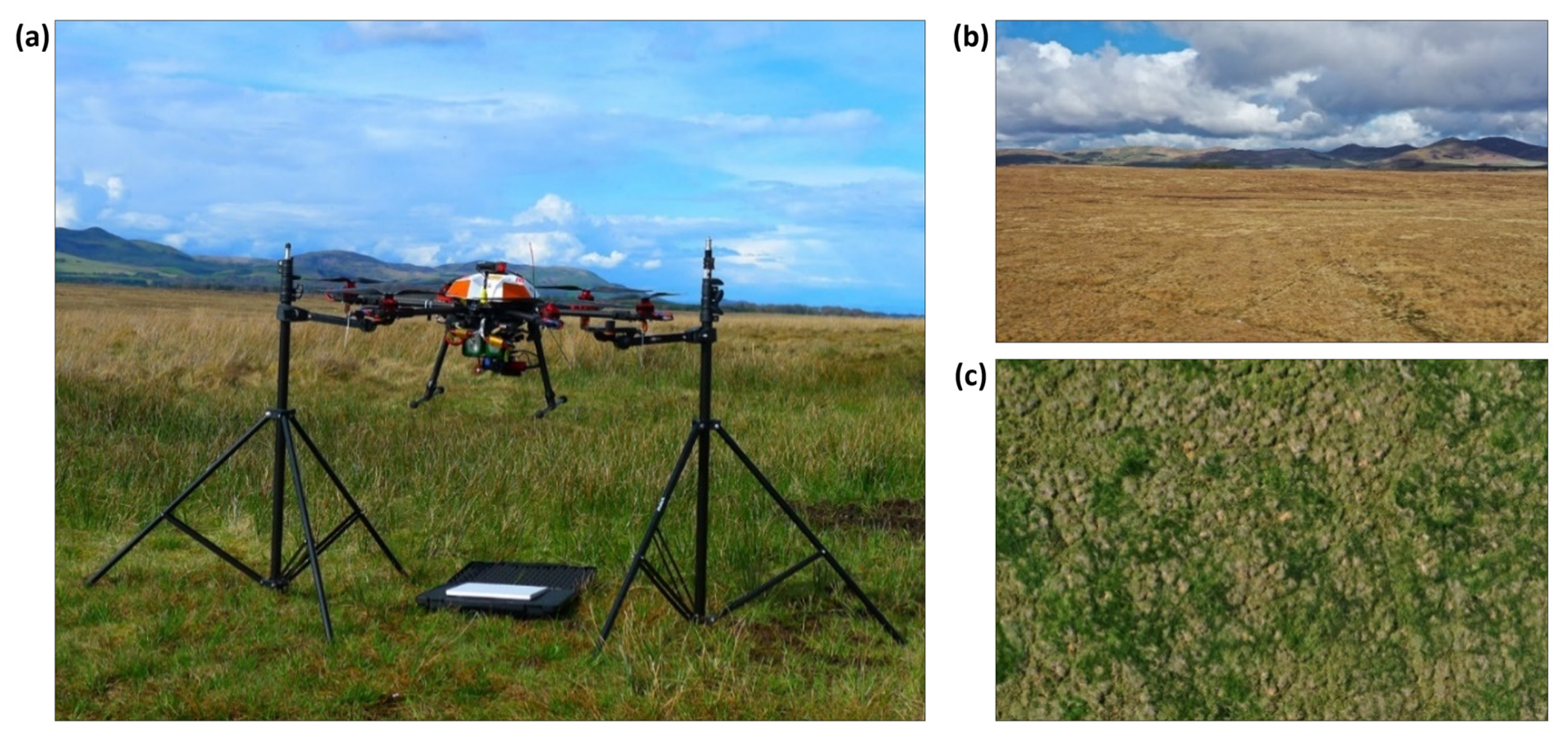
Figure 2.
Diurnal overview of the solar conditions on the multispectral survey days. Shown are: the period of UAV image acquisition (yellow shaded areas); half-hourly incoming photosynthetically active radiation (PAR) measured at the site (black dots; SKP215, Skye Instruments Ltd., Llandrindod Wells, UK), and solar zenith angle (blue line) calculated using the NOAA Solar Calculator (https://gml.noaa.gov/grad/solcalc/, accessed on 21 January 2022). From top to bottom are the survey days: 14 May (overcast), 2 June (clear), 23 July (clear), 3 August (overcast), 25 August (clear), 20 September (clear), and 15 October 2021 (clear).

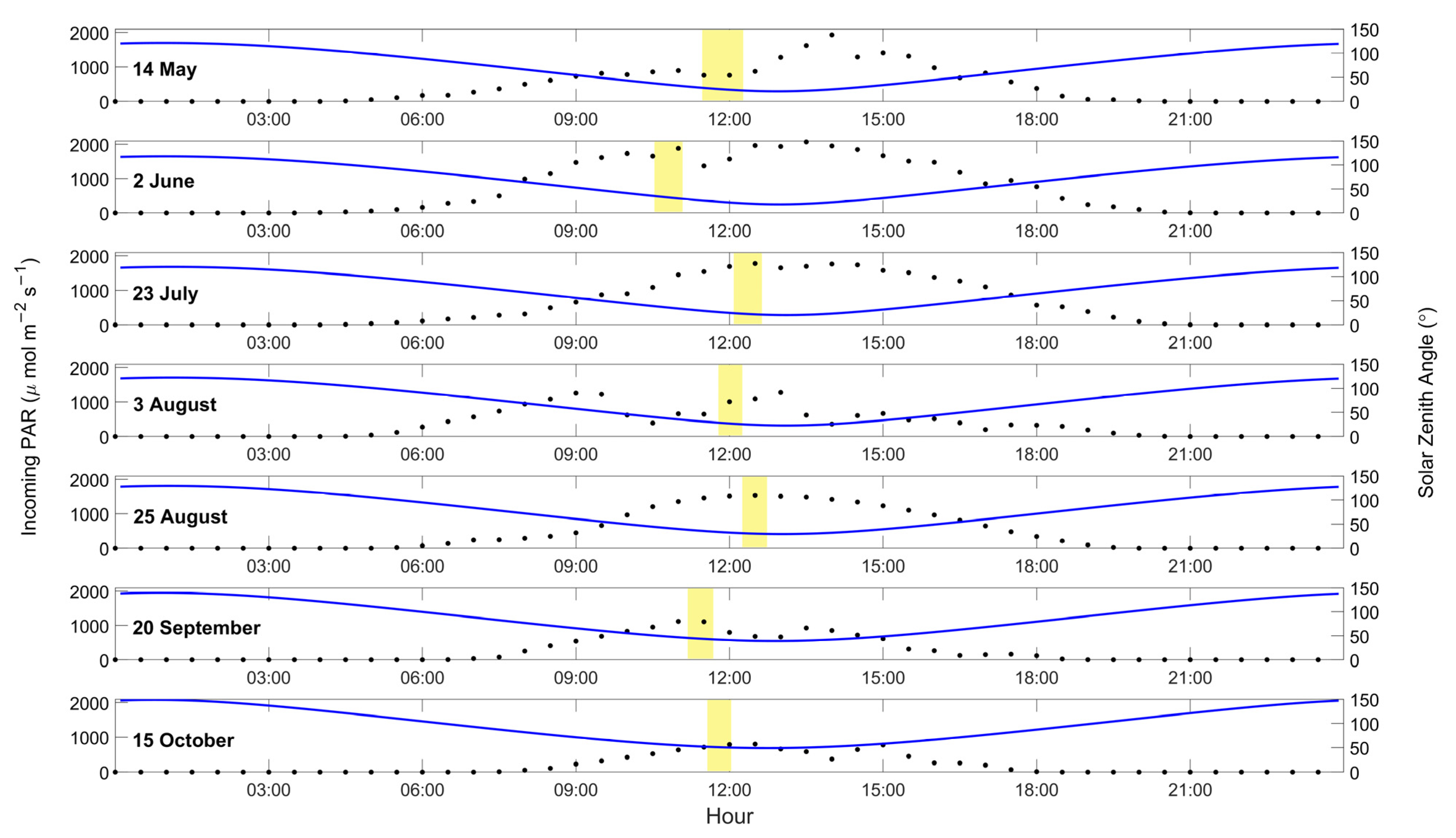
Figure 3.
Photographs of the eleven dominant upper-canopy species identified by the ground survey. Photo credit: G. Simpson.

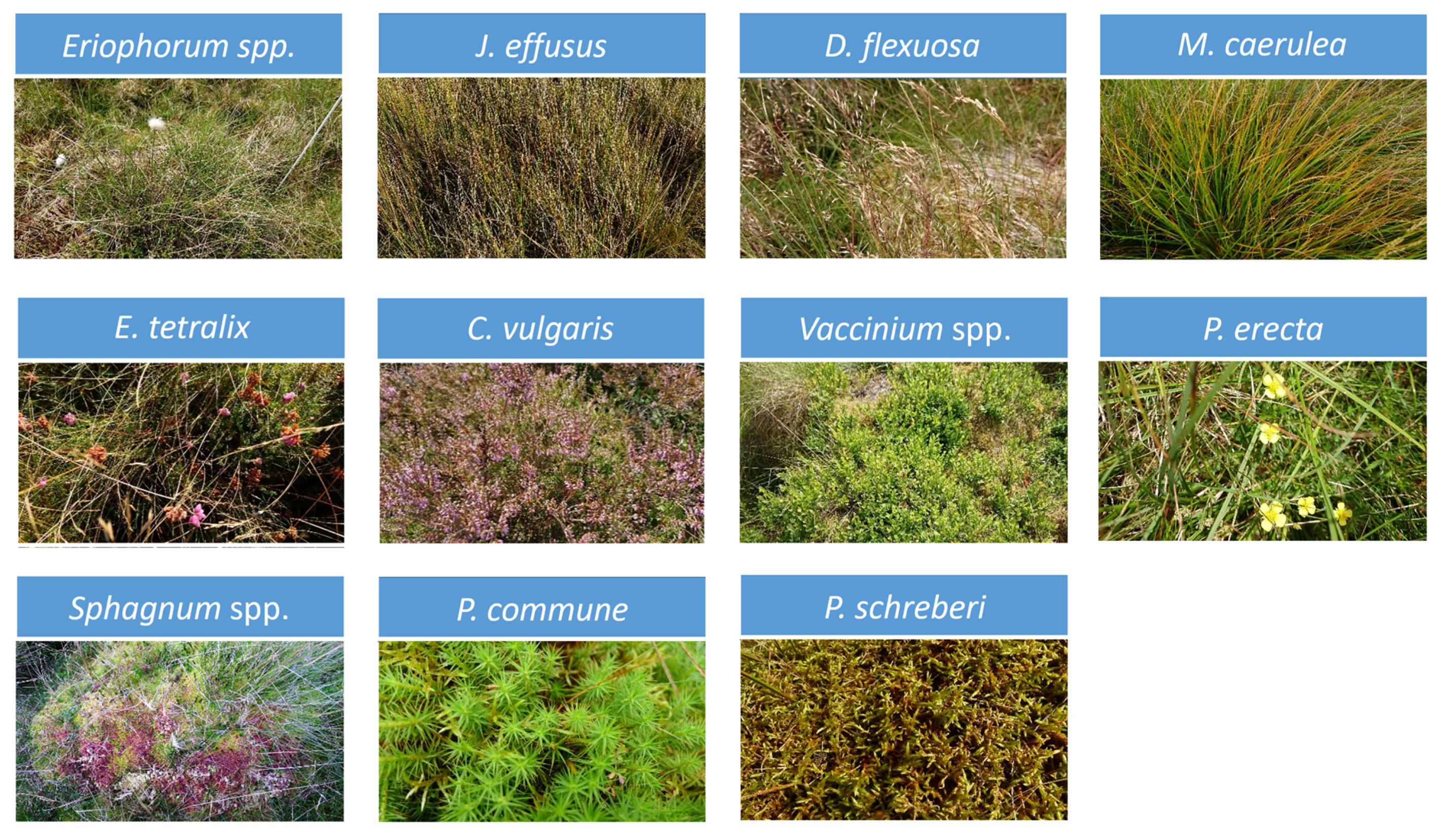
Figure 4.
Outline of the data used to explore the impact of the spatial and temporal resolutions of the UAV imagery on the classification accuracy.

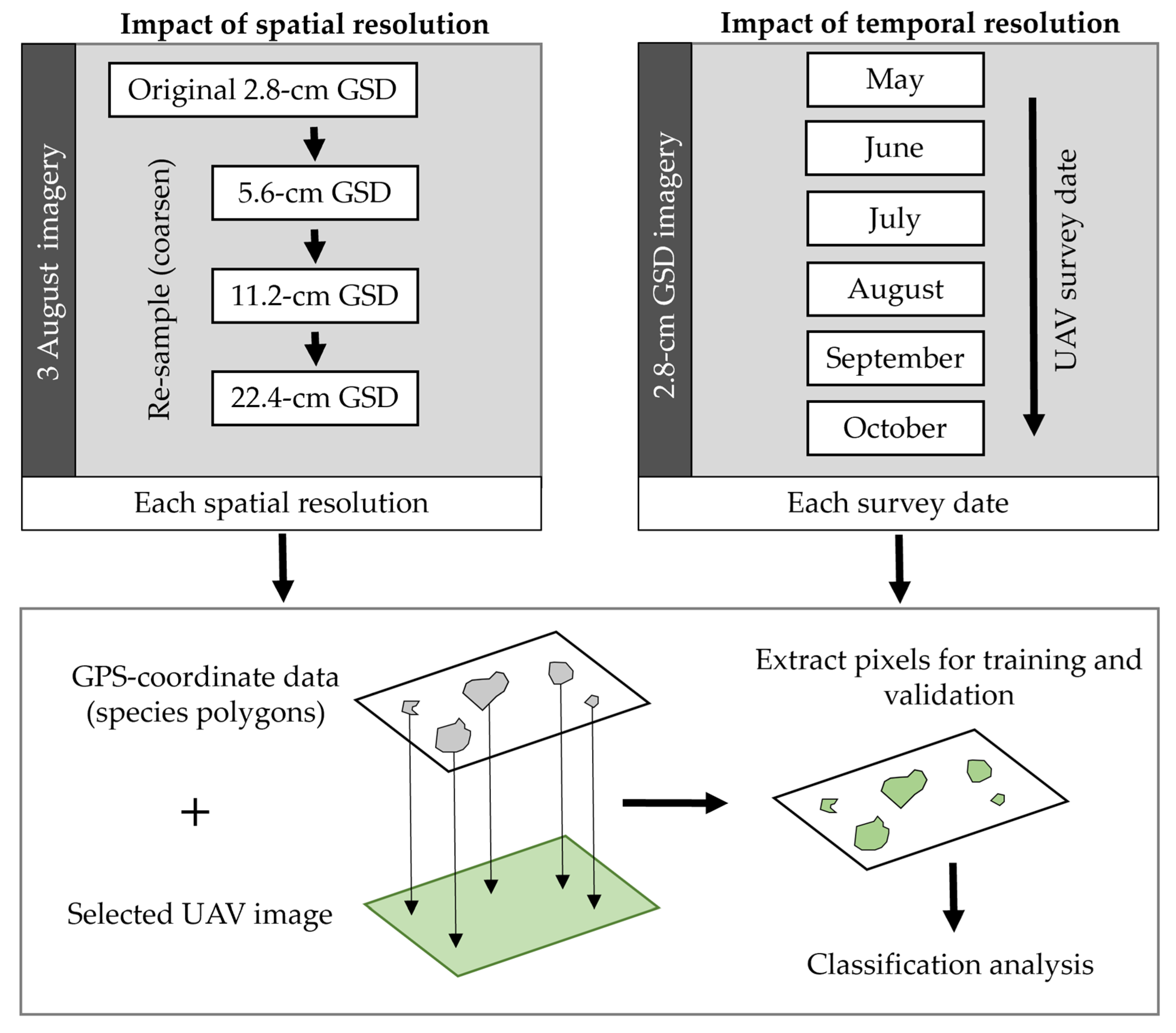
Figure 5.
RGB (true-colour composite, (a)) and multispectral (false-colour composite, (b); RGB = b4-b2-b1) orthomosaics of the study area taken on 3 August 2021. The RGB image on the left (a) shows the location of training (red) and validation (grey) data points used in the classification analysis.

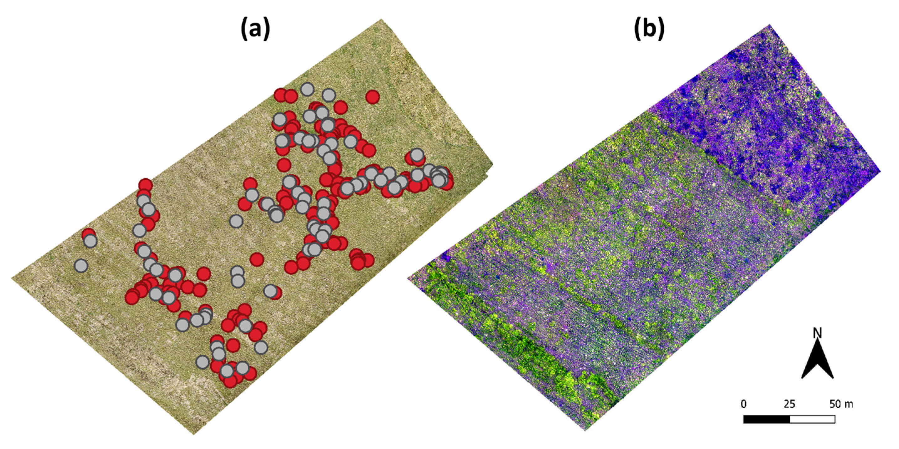
Figure 6.
Spectral signatures of the dominant vegetation species at Auchencorth Moss. The reflectance data shown are from the field spectroscopy measurements conducted with the ASD on 23 July 2021. The gaps in the presented spectra result from the removal of bands affected by noise and atmospheric water absorption features. The wavelengths sampled by the four Parrot Sequoia bands (green, red, red-edge, and NIR, respectively) are depicted by the vertical grey bars towards the left-hand side of the plot.

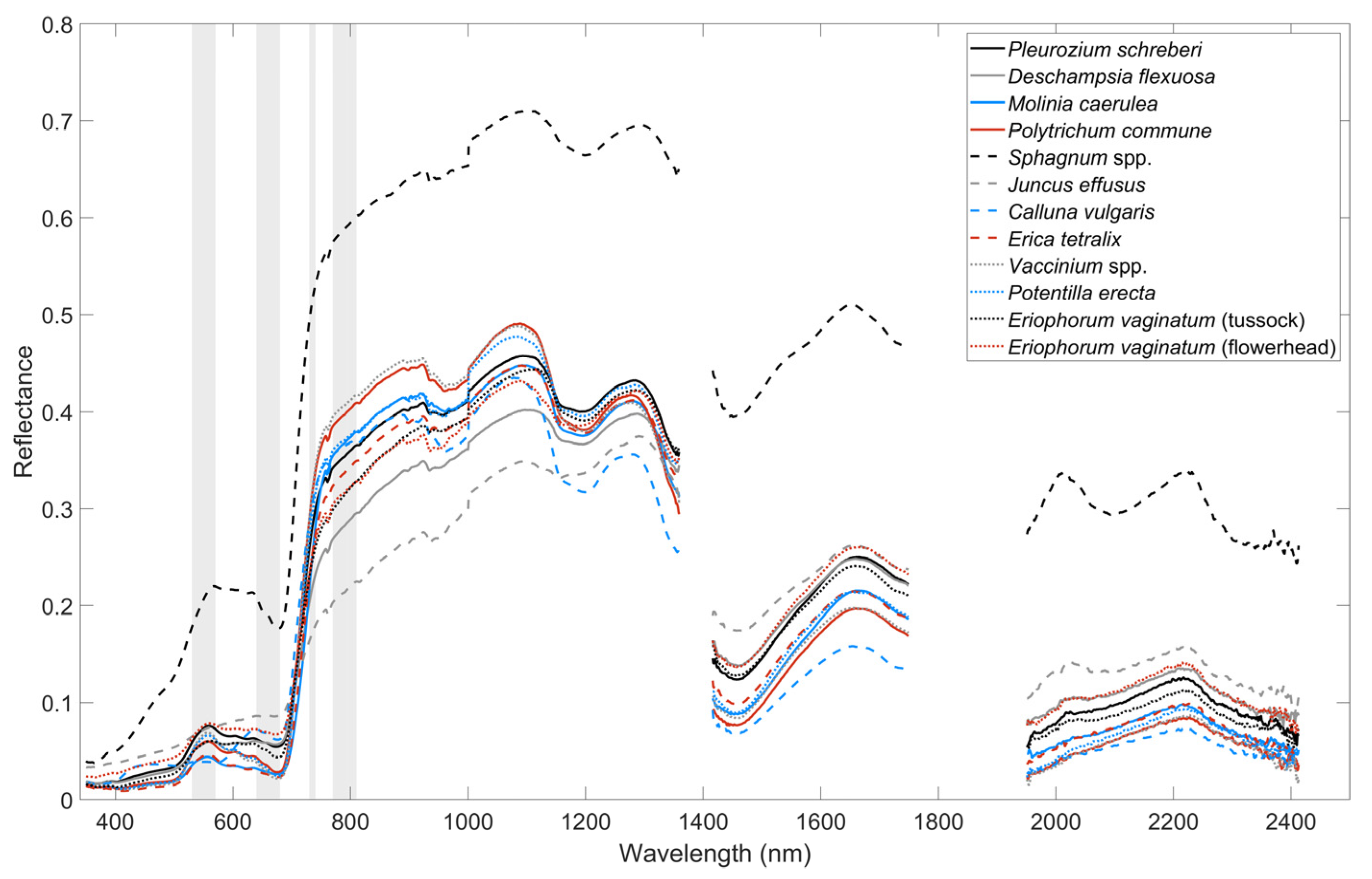
Figure 7.
Impact of the spatial resolution on the image classification. Shown are false-colour composites of the multispectral imagery (left; RGB = b4-b2-b1) used as input for the Maximum Likelihood (ML) classification (right; see legend). A coarsening image resolution is shown from top to bottom (2.8 cm GSD to 22.4 cm GSD). Note, these classifications were conducted using the GNSS survey point data for ground validation.

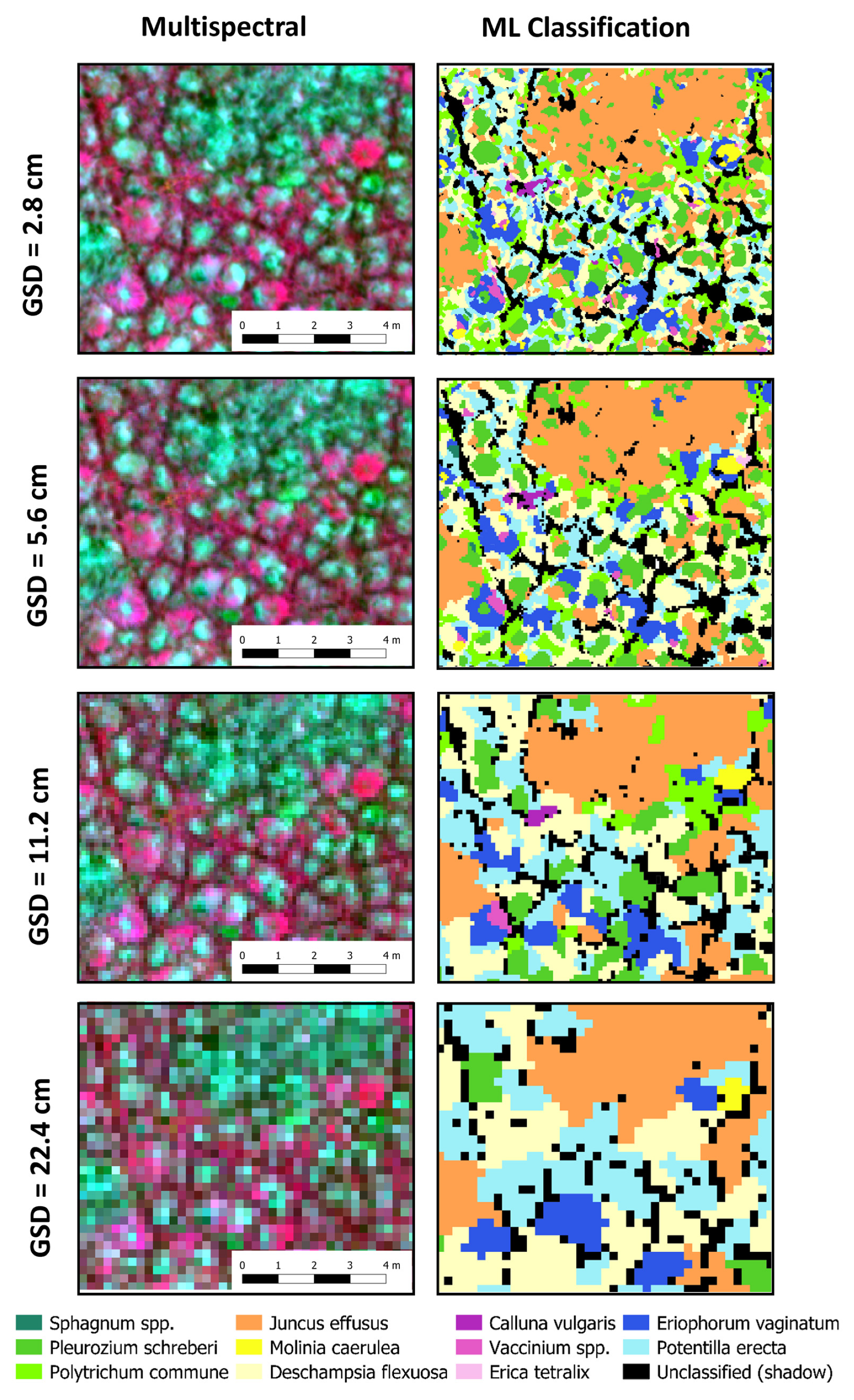
Figure 8.
Multispectral imagery of Auchencorth Moss over the 2021 growing season. Shown are false-colour composites (RGB = b4-b2-b1) of the survey area acquired on three dates: 14 May (a); 3 August (b); and 15 October (c).

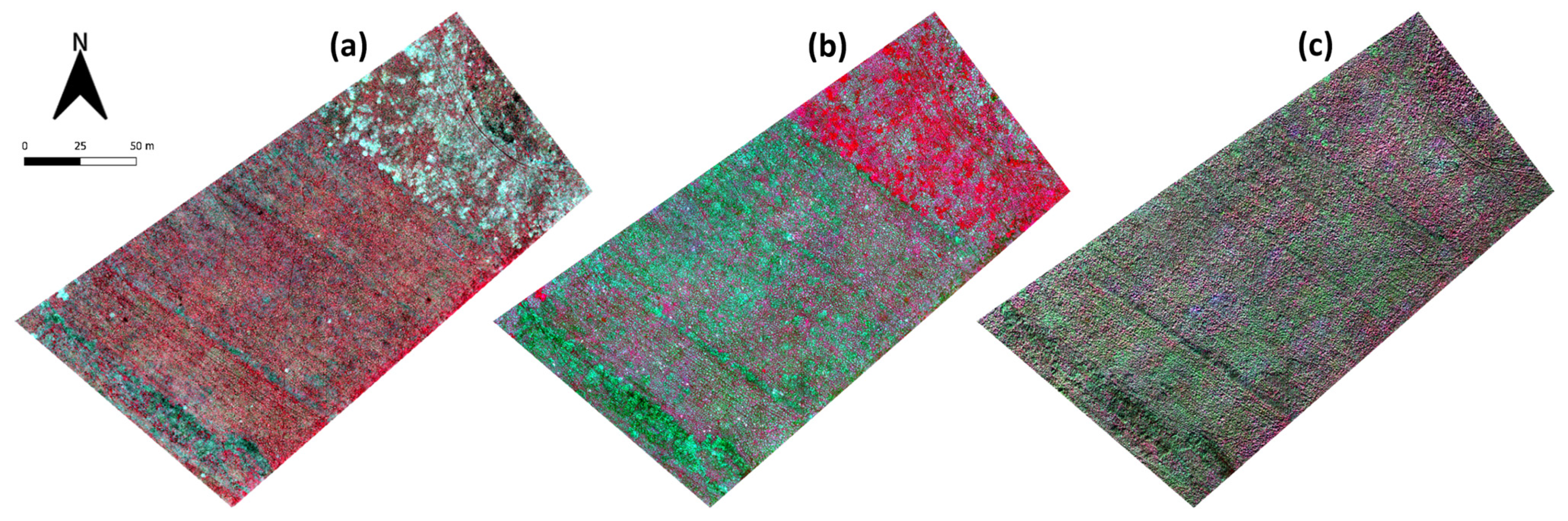
Figure 9.
Temporal vegetation classifications of Auchencorth Moss over the 2021 growing season. Shown are the results of the Maximum Likelihood (ML) classifier run with imagery acquired on 14 May (a); 3 August (b); and 15 October (c). Note, the presented classifications varied in accuracy and were conducted using the GNSS survey point data for ground validation.

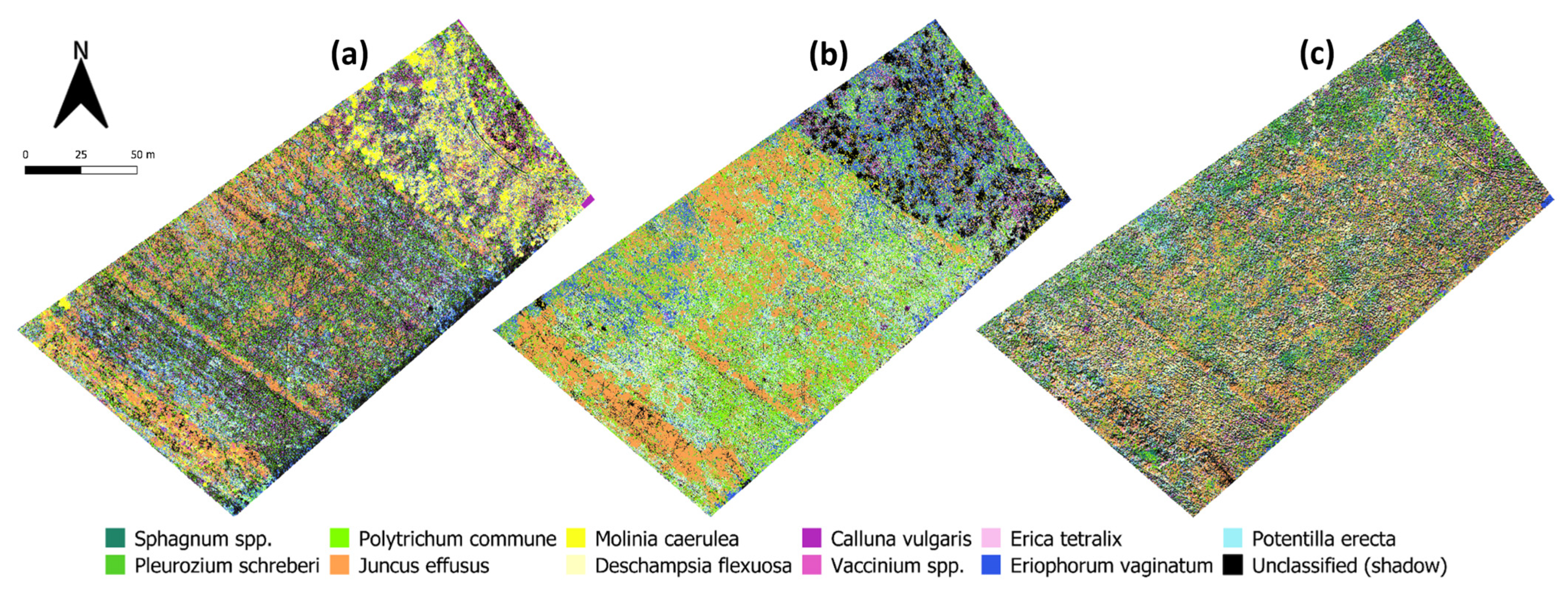
Table 1.
Overview of the types of UAV data collected at Auchencorth Moss during the 2021 growing season. Ground sampling distance (GSD) describes the physical distance between adjacent pixel centres in the imagery, i.e., for a 2 cm GSD each pixel corresponds to a 2 cm distance on the ground. The accuracy of each dataset is indicated by the calculated root mean square error (RMSE) values. Hereby, the observed locations of five Check Points (CPs) in the processed imagery were compared against their corresponding ground-surveyed GNSS (Global Navigation Satellite System) coordinates. Note that these CPs were not used during image processing and hence provide an independent assessment of the geolocation accuracy in the processed imagery. For the multispectral data, the GSD and RMSE represent mean values (averaged over all flights during the growing season); for the RGB imagery, data were employed from a single survey conducted on 18 May 2021.

Sensor	Data Type	Survey Height (m)	Image Overlap (% Front, Side)	GSD (cm)	RMSE [x, y, z] (cm)
Mavic Pro 2	RGB	65	70, 80	1.46	1.12
					0.97
					4.07
Parrot Sequoia	Multispectral	25	80, 80	2.80	1.35
					1.47
					6.50

Table 2.
Size of the ‘dominant species’ regions of interest (ROIs) collected for training the classification models and validating the outputs. Shown are the total number of polygons surveyed for each ROI and the total number of pixels contained therein.

ROI Class	Total No. Polygons	Total No. Pixels
Eriophorum vaginatum	39	11,361
Juncus effusus	18	27,887
Deschampsia flexuosa	23	7118
Molinia caerulea	25	25,284
Erica tetralix	20	3442
Calluna vulgaris	19	8358
Vaccinium spp.	16	3524
Potentilla erecta	19	882
Sphagnum spp.	11	2157
Polytrichum commune	32	7264
Pleurozium schreberi	34	8666
SUM	256	105,943

Table 3.
Confusion matrix based on a Maximum Likelihood (ML) classification of the peak growing season imagery (3 August 2021). The analysis was conducted using original resolution data (2.8 cm GSD) in a 5-band image stack (multispectral and normalised DSM data), and GNSS survey point data were employed for the ground validation. Columns represent ground validation data, and rows represent classification output based on the training data. Note, values in the table’s centre denote the number of pixels, with those in bold along the diagonal indicating the number of pixels for which the classification predicted the same species as in the ground validation data. The User and Producer accuracy are given as percentage values for ease of reference, with overall classification accuracy indicated in bold.

		Ground Validation Data
		P. schreberi	D. flexuosa	M. caerulea	P. commune	Sphagnum spp.	J. effusus	C. vulgaris	E. tetralix	Vaccinium spp.	P. erecta	E. vaginatum	User Acc.
Classification output	P. schreberi	1544	54	26	31	0	258	7	23	0	1	267	70%
	D. flexuosa	153	1181	240	107	0	1	38	154	1	54	728	45%
	M. caerulea	0	0	1023	0	0	0	0	0	50	0	606	61%
	P. commune	12	196	71	684	3	190	53	17	0	43	13	53%
	Sphagnum spp.	54	1	0	0	462	0	0	0	0	0	8	88%
	J. effusus	196	64	0	421	0	6412	0	0	7	23	63	89%
	C. vulgaris	0	0	19	35	0	0	1202	17	21	0	0	93%
	E. tetralix	10	15	16	0	0	0	195	687	0	0	38	72%
	Vaccinium spp.	0	0	23	13	0	0	0	0	897	26	235	75%
	P. erecta	114	361	70	160	9	174	34	23	0	85	358	6%
	E. vaginatum	130	31	206	38	48	33	9	2	14	29	1091	67%
	Producer Acc.	70%	62%	60%	46%	89%	91%	78%	74%	91%	33%	32%	69%

Table 4.
Impact of the spatial resolution on the classification accuracy. Shown are accuracy statistics for a Maximum Likelihood (ML) classifier run with imagery collected on 3 August 2021, employing GNSS point data as ground validation. The original 2.8 cm GSD dataset was resampled to produce three sets of coarser resolution imagery used in the classification.

Spatial Resolution	Classification Accuracy
Spatial Resolution	Overall Accuracy	Kappa Coefficient
2.8 cm GSD	68.5%	0.63
5.6 cm GSD	65.4%	0.60
11.2 cm GSD	64.9%	0.59
22.4 cm GSD	42.8%	0.35

[ad_2]