Fueling the Future: A Comprehensive Analysis and Forecast of Fuel Consumption Trends in U.S. Electricity Generation
[ad_1]
Author Contributions
Conceptualization, M.M.H.B.; methodology, M.M.H.B.; software, M.M.H.B.; validation, M.M.H.B. and T.R.; formal analysis, M.M.H.B.; investigation, M.M.H.B.; resources, M.M.H.B.; writing—original draft preparation, M.M.H.B. and A.N.S.; writing—review and editing, T.R., S.I.A. and A.N.S.; visualization, supervision, T.R. and M.M.H.B.; project administration, A.N.S. and M.M.H.B. All authors have read and agreed to the published version of the manuscript.
Figure 1.
Trend analysis of different fuels’ consumption for U.S. electricity generation over time.
Figure 1.
Trend analysis of different fuels’ consumption for U.S. electricity generation over time.
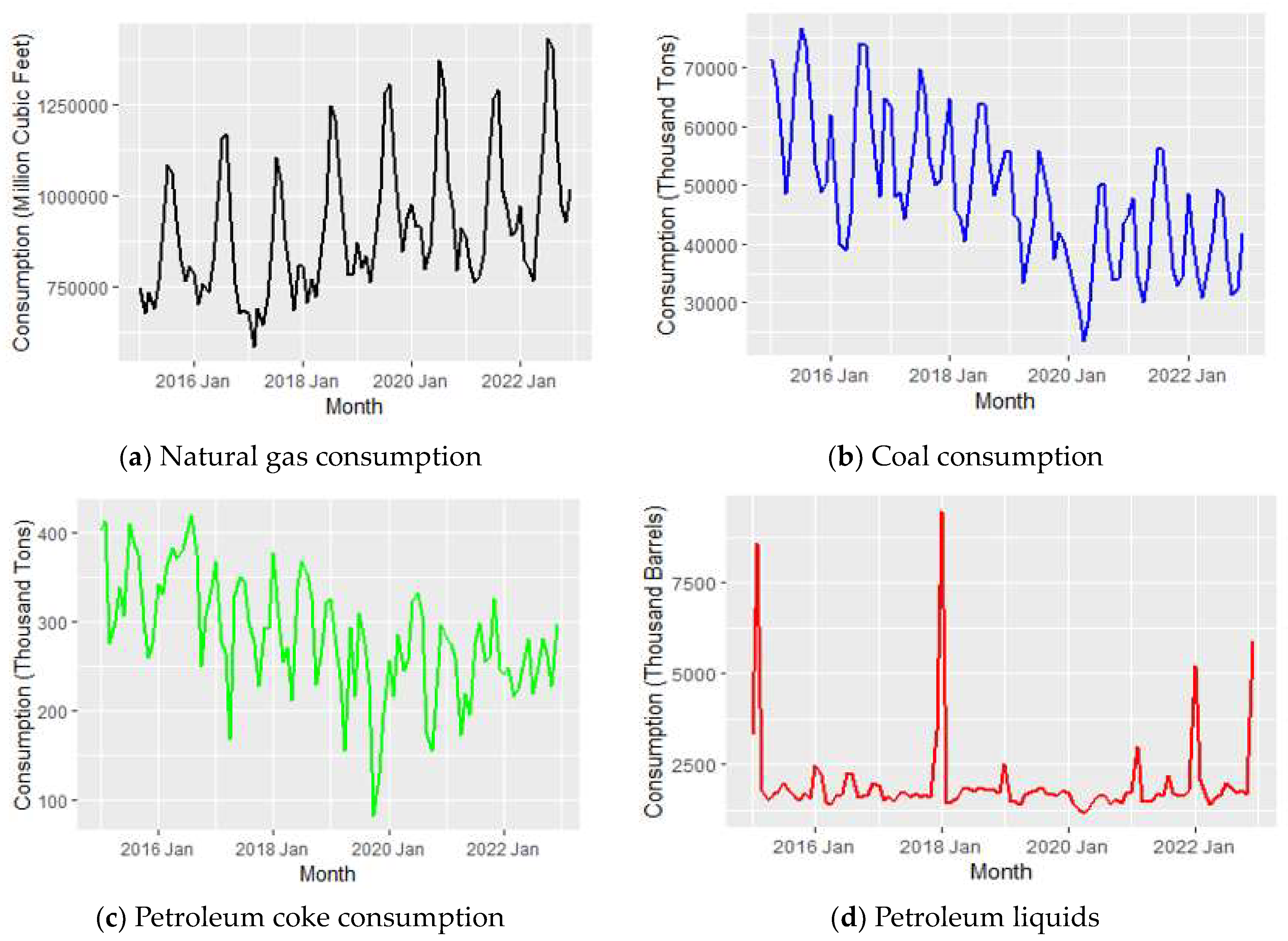
Figure 2.
Monthly consumption and seasonality analysis of NG from 2015 to 2022.
Figure 2.
Monthly consumption and seasonality analysis of NG from 2015 to 2022.
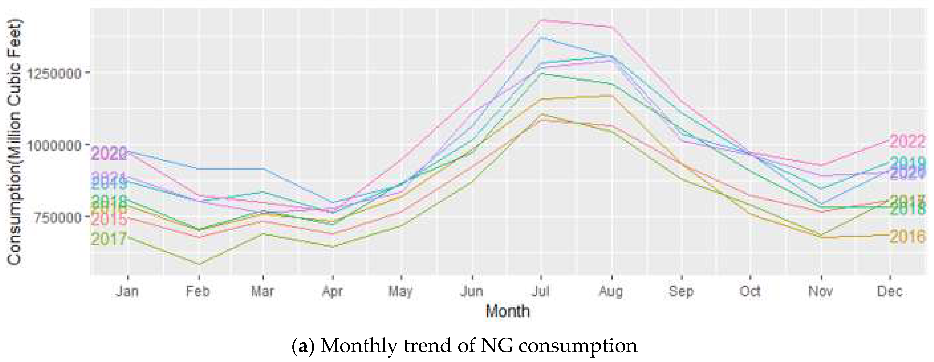
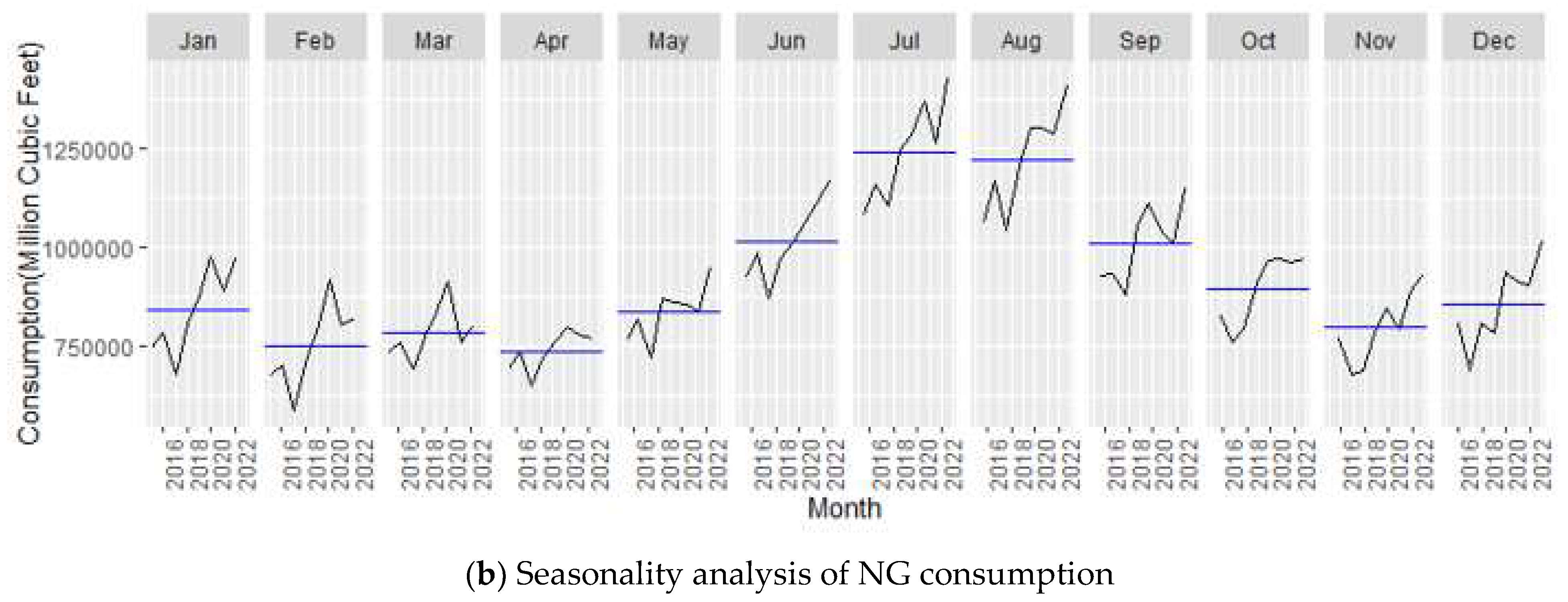
Figure 3.
Monthly consumption and seasonality analysis of coal from 2015 to 2022.
Figure 3.
Monthly consumption and seasonality analysis of coal from 2015 to 2022.
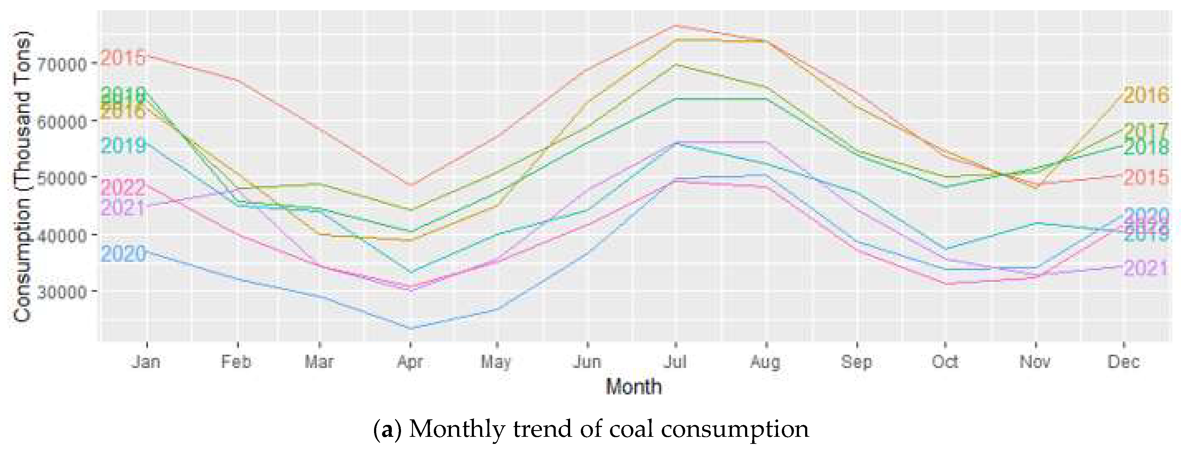
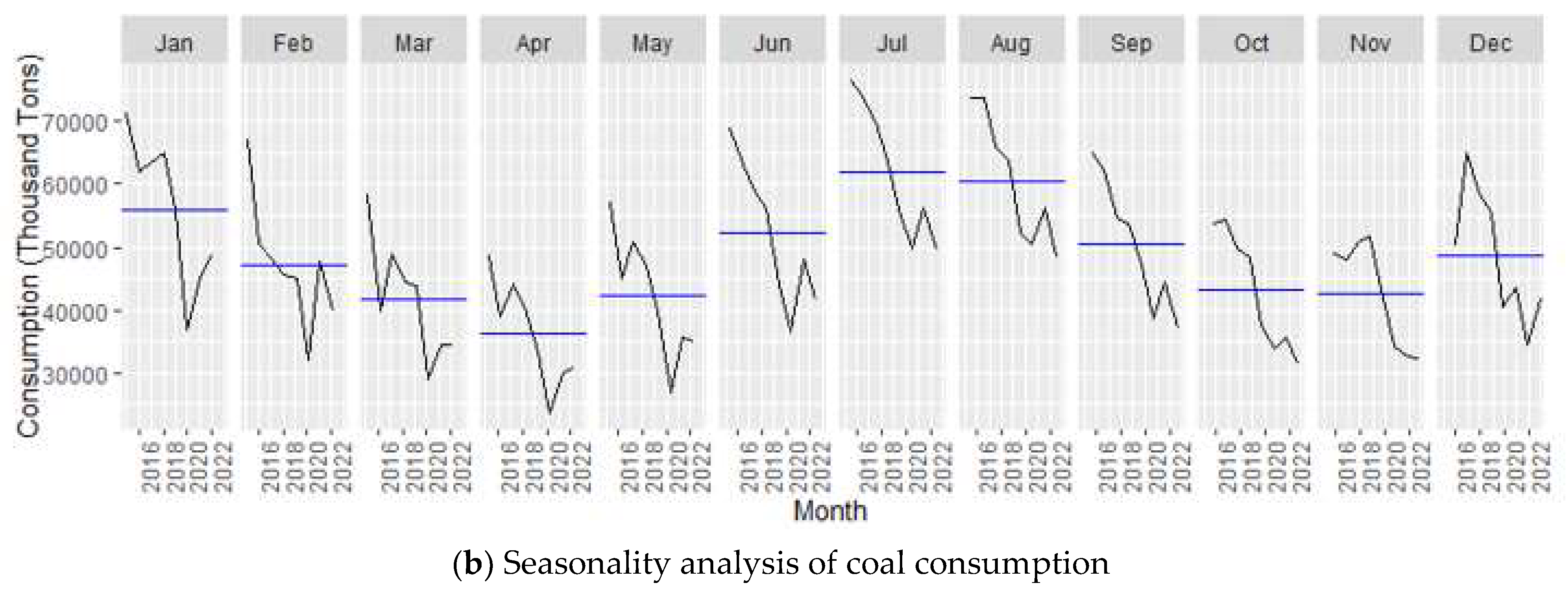
Figure 4.
Monthly consumption and seasonality analysis of petroleum coke from 2015 to 2022.
Figure 4.
Monthly consumption and seasonality analysis of petroleum coke from 2015 to 2022.
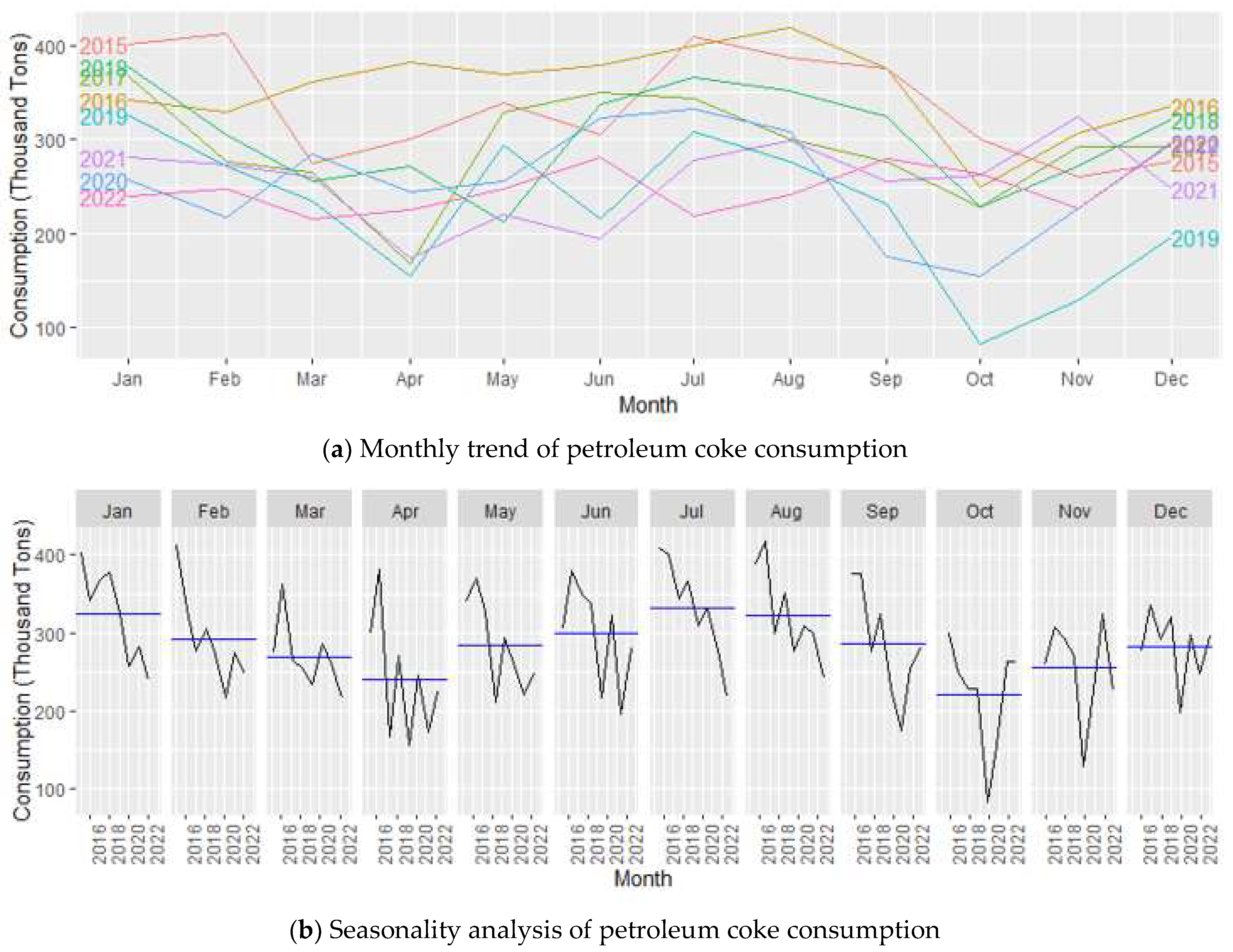
Figure 5.
Monthly consumption and seasonality analysis of petroleum liquids from 2015 to 2022.
Figure 5.
Monthly consumption and seasonality analysis of petroleum liquids from 2015 to 2022.
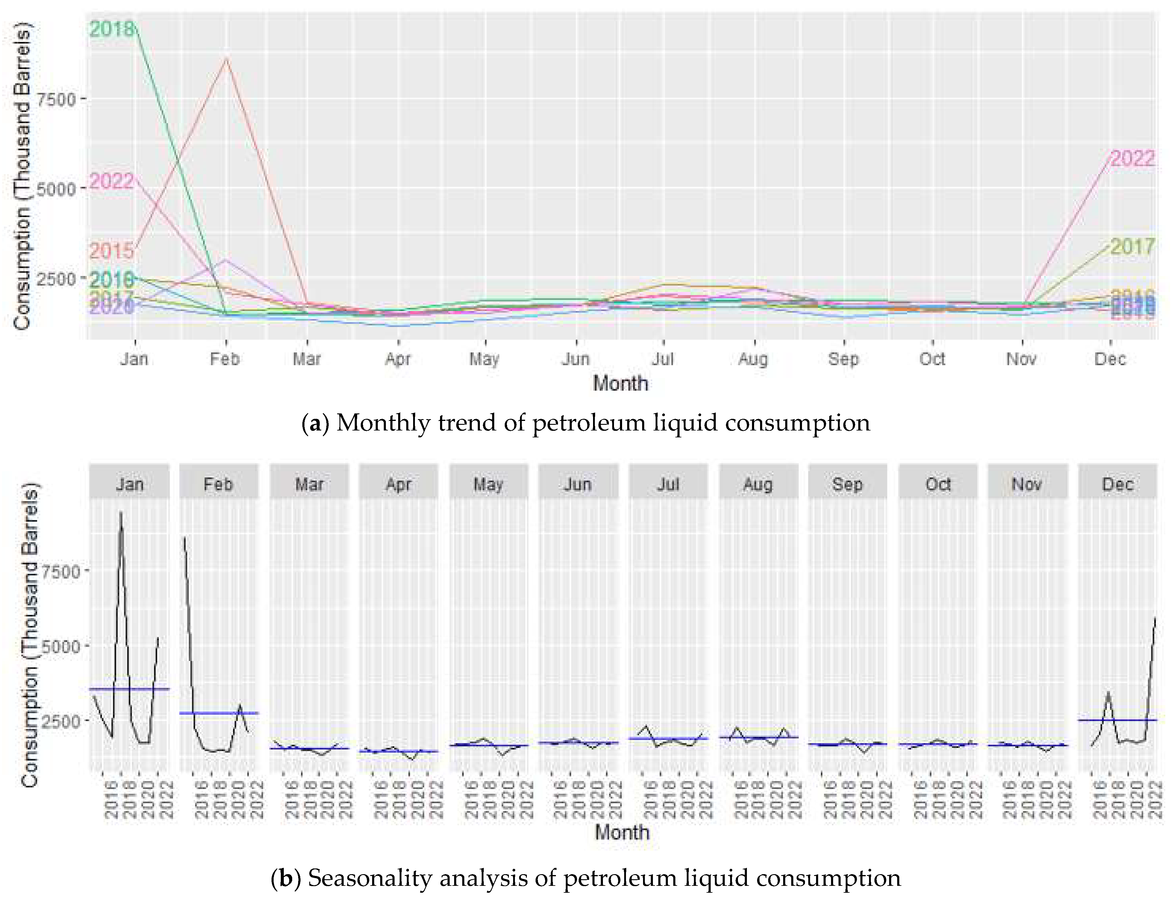
Figure 6.
Autocorrelation analysis of NG consumption using ACF and PACF plots. (a) ACF plot, NG consumption; (b) PACF plot, NG consumption.
Figure 6.
Autocorrelation analysis of NG consumption using ACF and PACF plots. (a) ACF plot, NG consumption; (b) PACF plot, NG consumption.
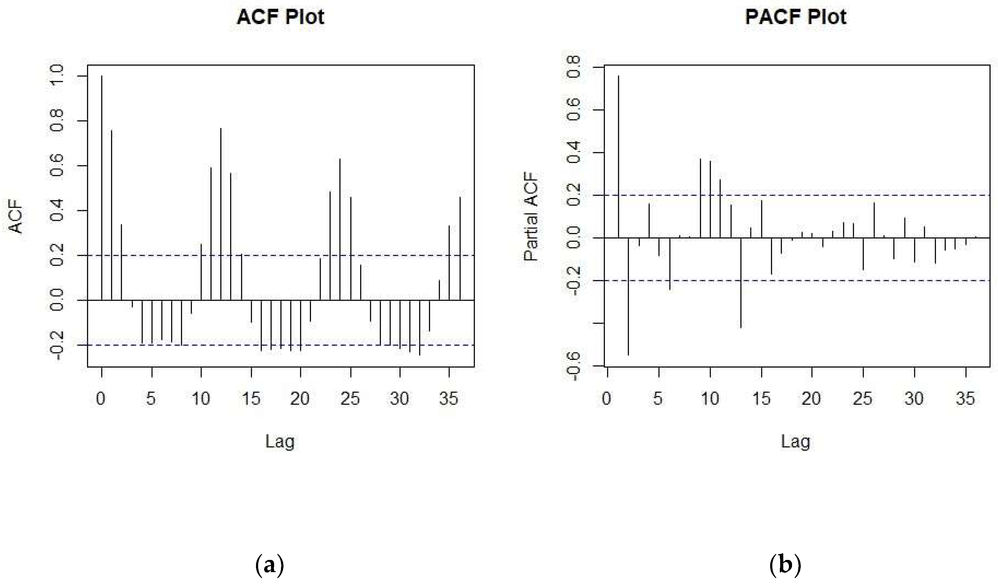
Figure 7.
Autocorrelation analysis of coal consumption using ACF and PACF plots. (a) ACF plot, coal consumption; (b) PACF plot, coal consumption.
Figure 7.
Autocorrelation analysis of coal consumption using ACF and PACF plots. (a) ACF plot, coal consumption; (b) PACF plot, coal consumption.
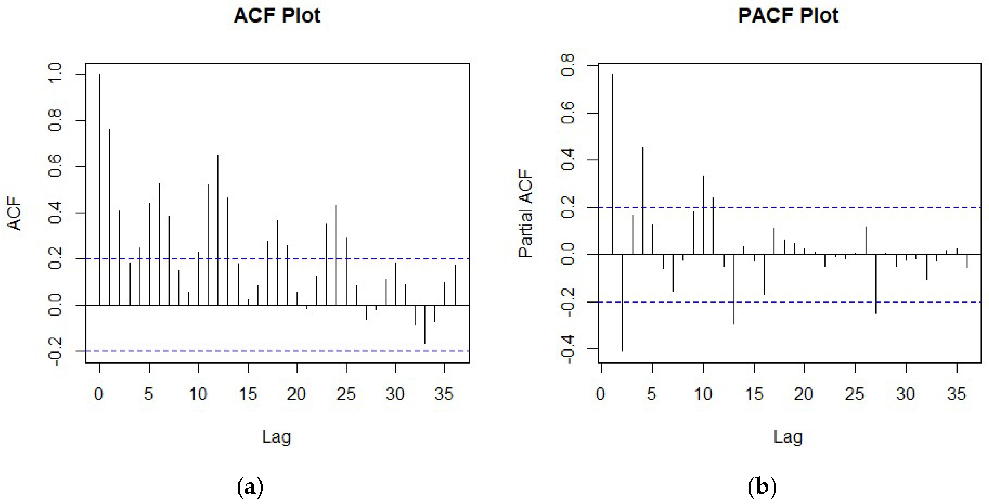
Figure 8.
Autocorrelation analysis of coal consumption using ACF and PACF plots. (a) ACF plot, petroleum coke consumption; (b) PACF plot, petroleum coke consumption.
Figure 8.
Autocorrelation analysis of coal consumption using ACF and PACF plots. (a) ACF plot, petroleum coke consumption; (b) PACF plot, petroleum coke consumption.
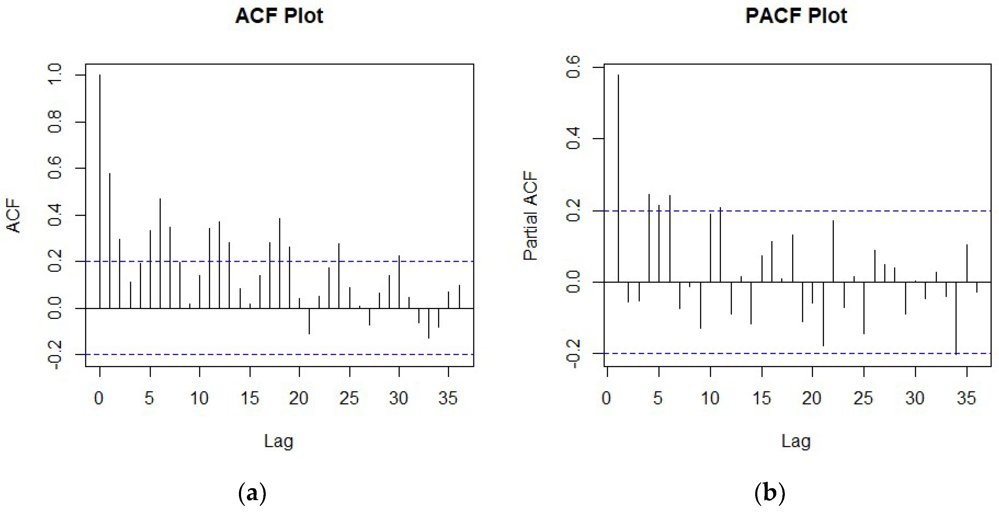
Figure 9.
Autocorrelation analysis of petroleum liquid using ACF and PACF plots. (a) ACF plot, petroleum liquid consumption; (b) PACF plot, petroleum liquid consumption.
Figure 9.
Autocorrelation analysis of petroleum liquid using ACF and PACF plots. (a) ACF plot, petroleum liquid consumption; (b) PACF plot, petroleum liquid consumption.
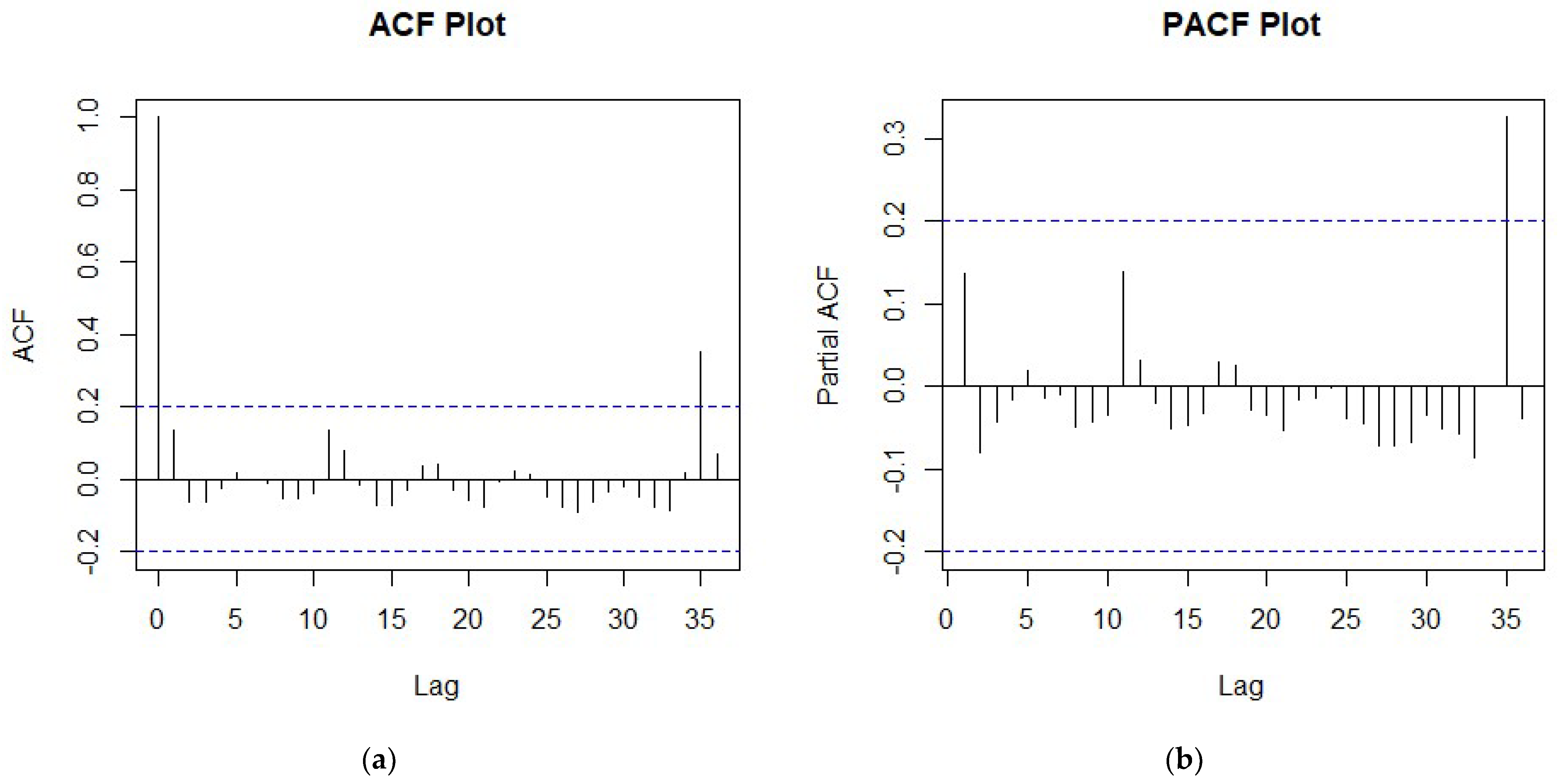
Figure 10.
Forecasting NG consumption for the years 2023 and 2024 using different forecasting methods.
Figure 10.
Forecasting NG consumption for the years 2023 and 2024 using different forecasting methods.
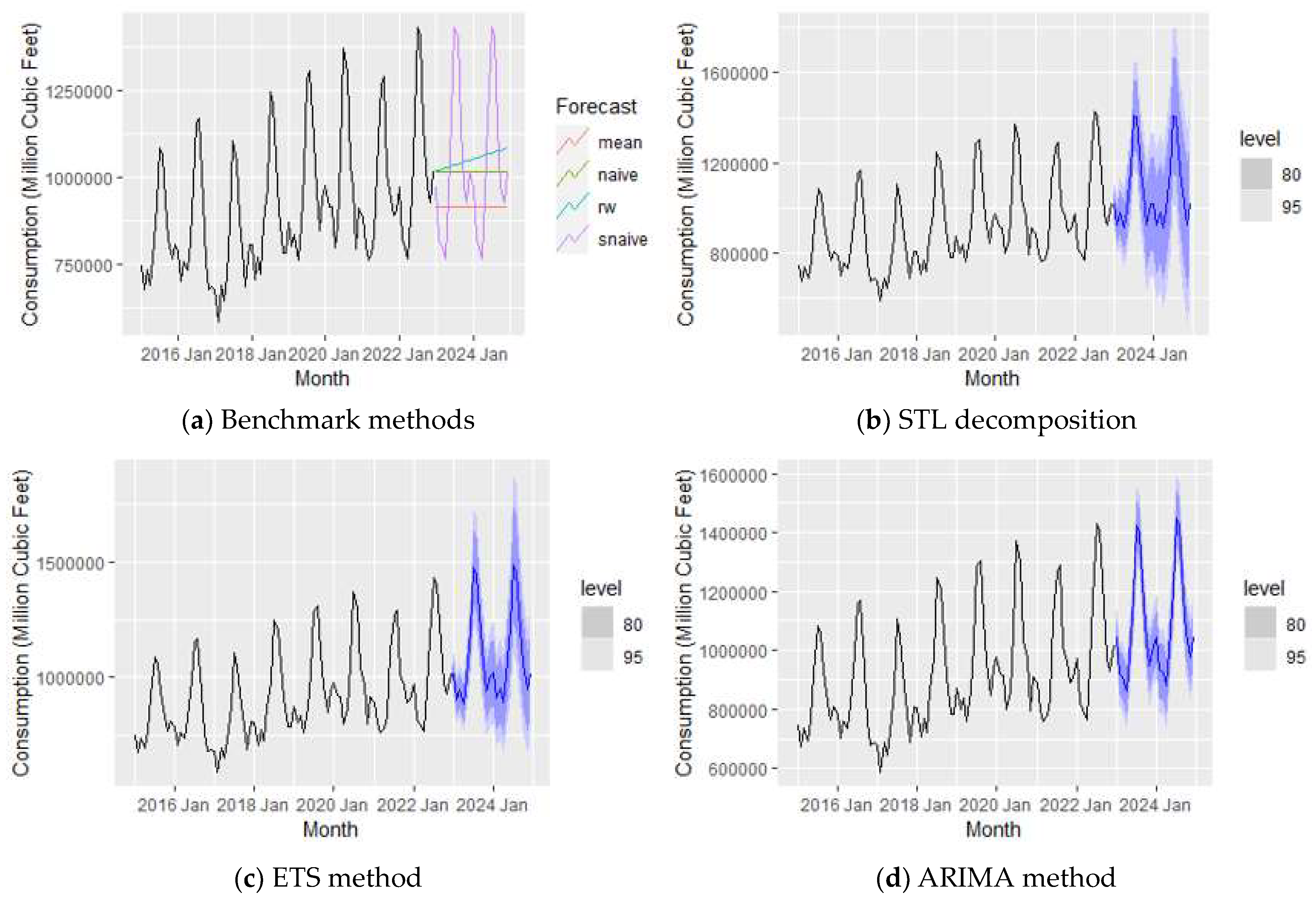
Figure 11.
ETS (M, N, M) decomposition plot of NG consumption.
Figure 11.
ETS (M, N, M) decomposition plot of NG consumption.
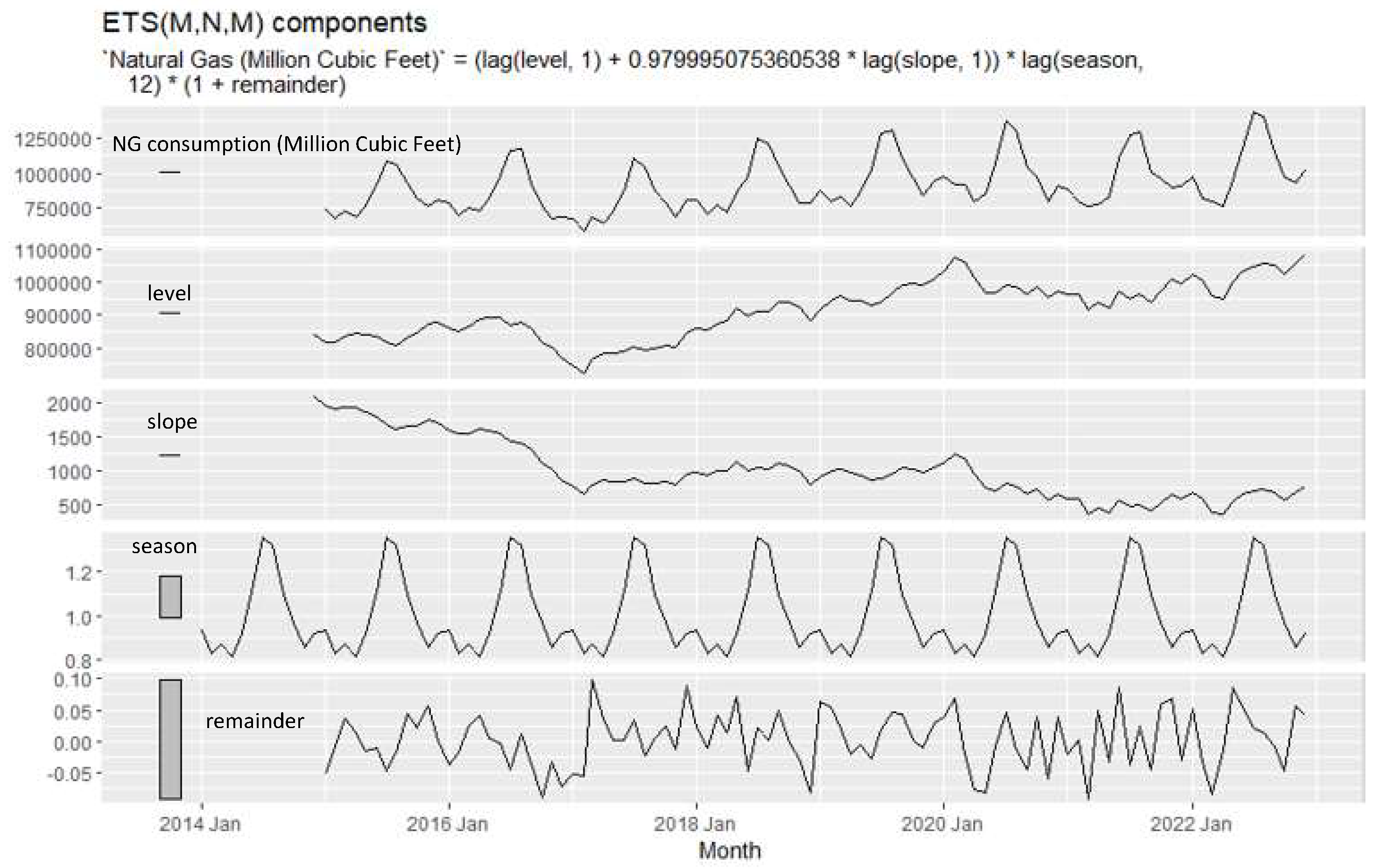
Figure 12.
Forecasting coal consumption for the years 2023 and 2024 using different forecasting methods.
Figure 12.
Forecasting coal consumption for the years 2023 and 2024 using different forecasting methods.
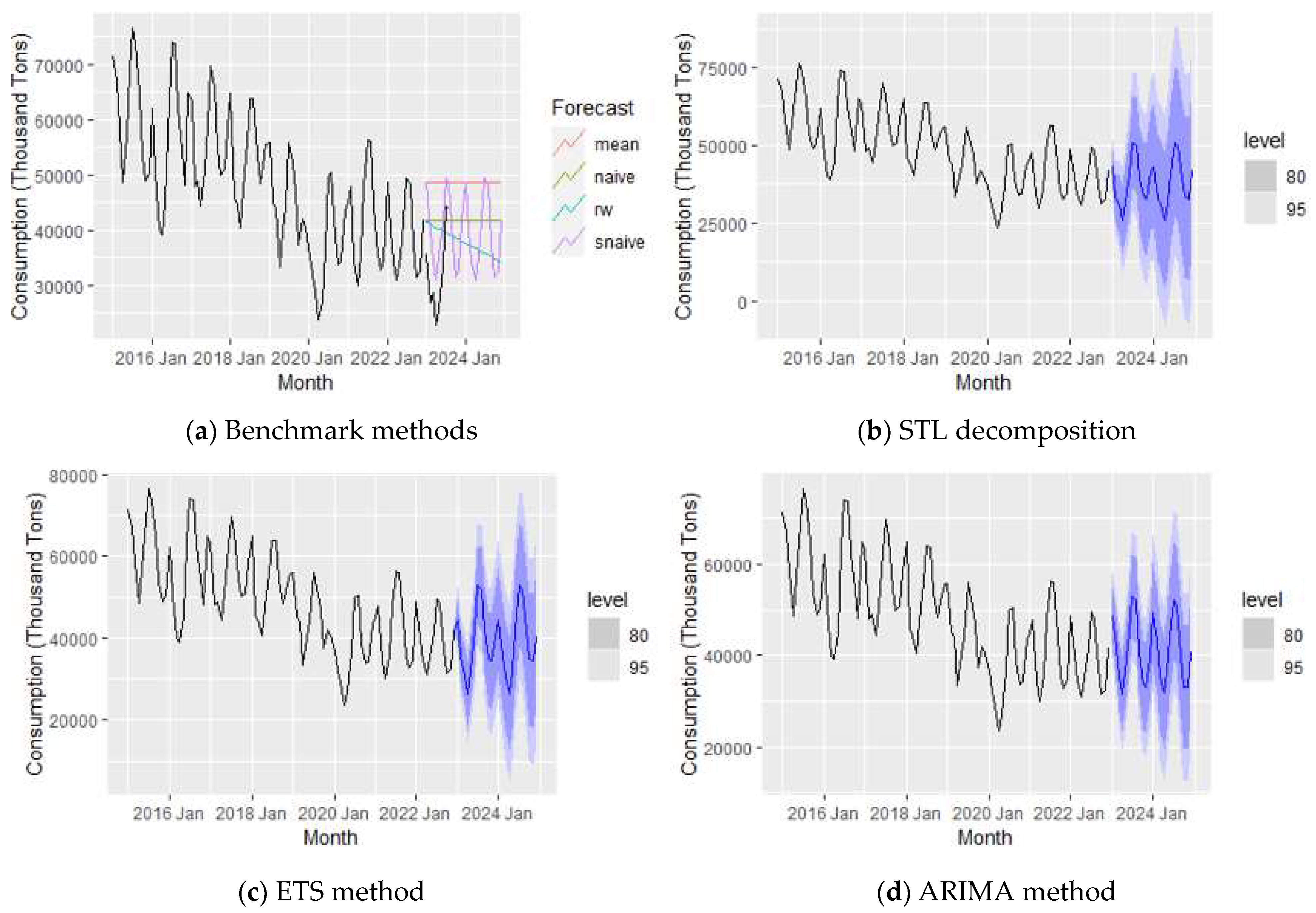
Figure 13.
Forecasting petroleum coke consumption for the years 2023 and 2024.
Figure 13.
Forecasting petroleum coke consumption for the years 2023 and 2024.
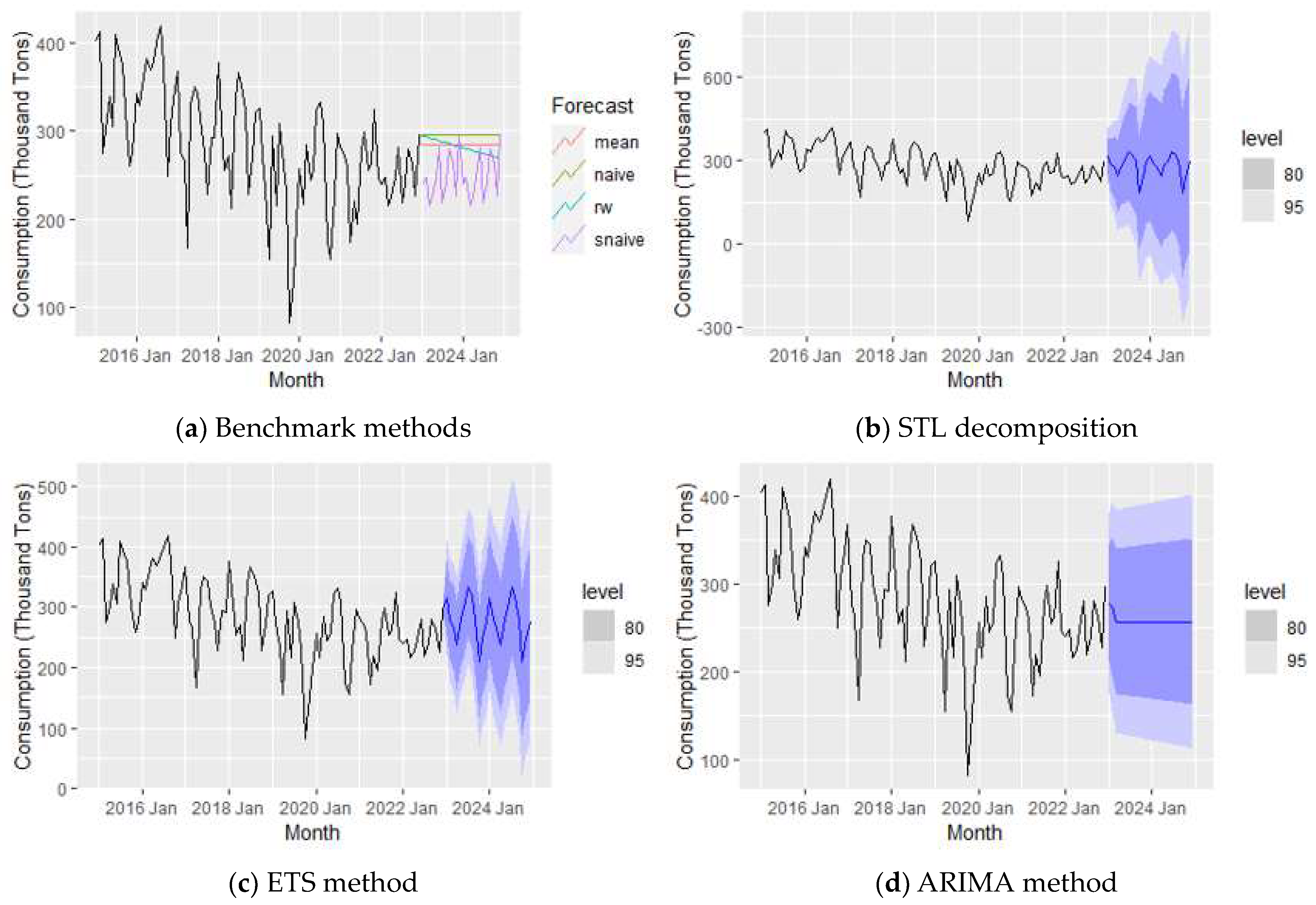
Figure 14.
Forecasting petroleum liquid consumption for the years 2023 and 2024.
Figure 14.
Forecasting petroleum liquid consumption for the years 2023 and 2024.
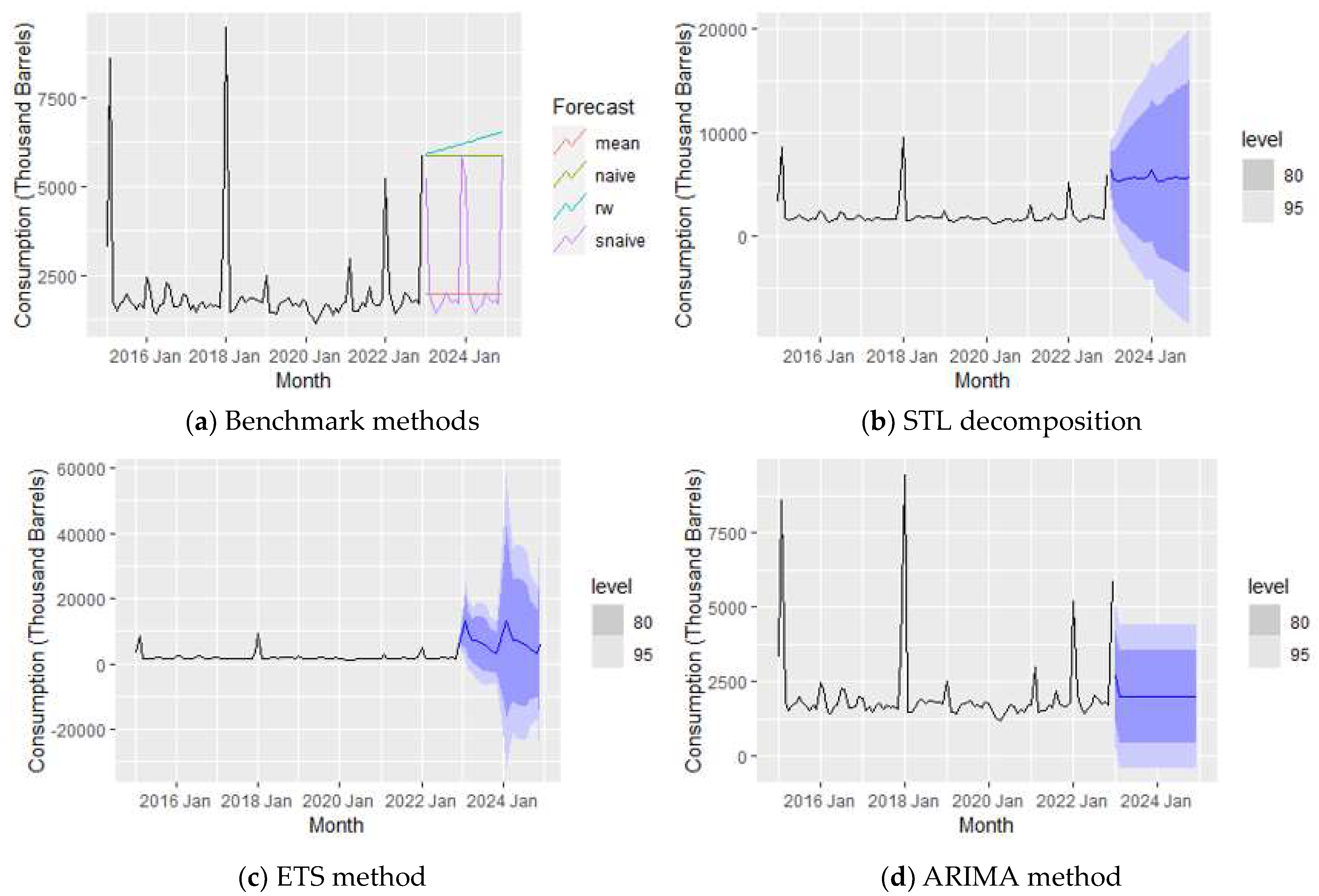
Figure 15.
Residual analysis of ETS forecasting method.
Figure 15.
Residual analysis of ETS forecasting method.
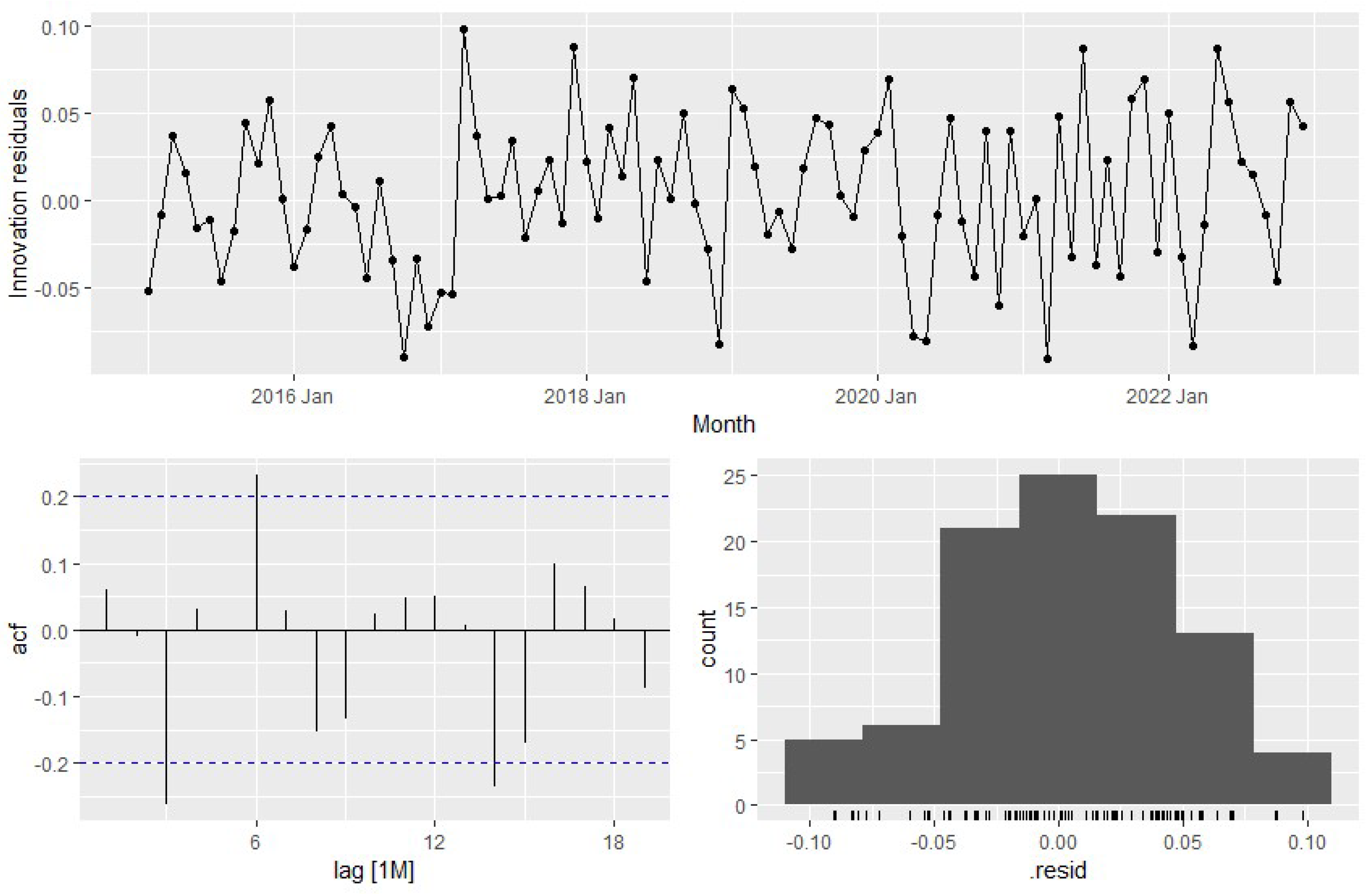
Figure 16.
Residual analysis of STLF forecasting method.
Figure 16.
Residual analysis of STLF forecasting method.
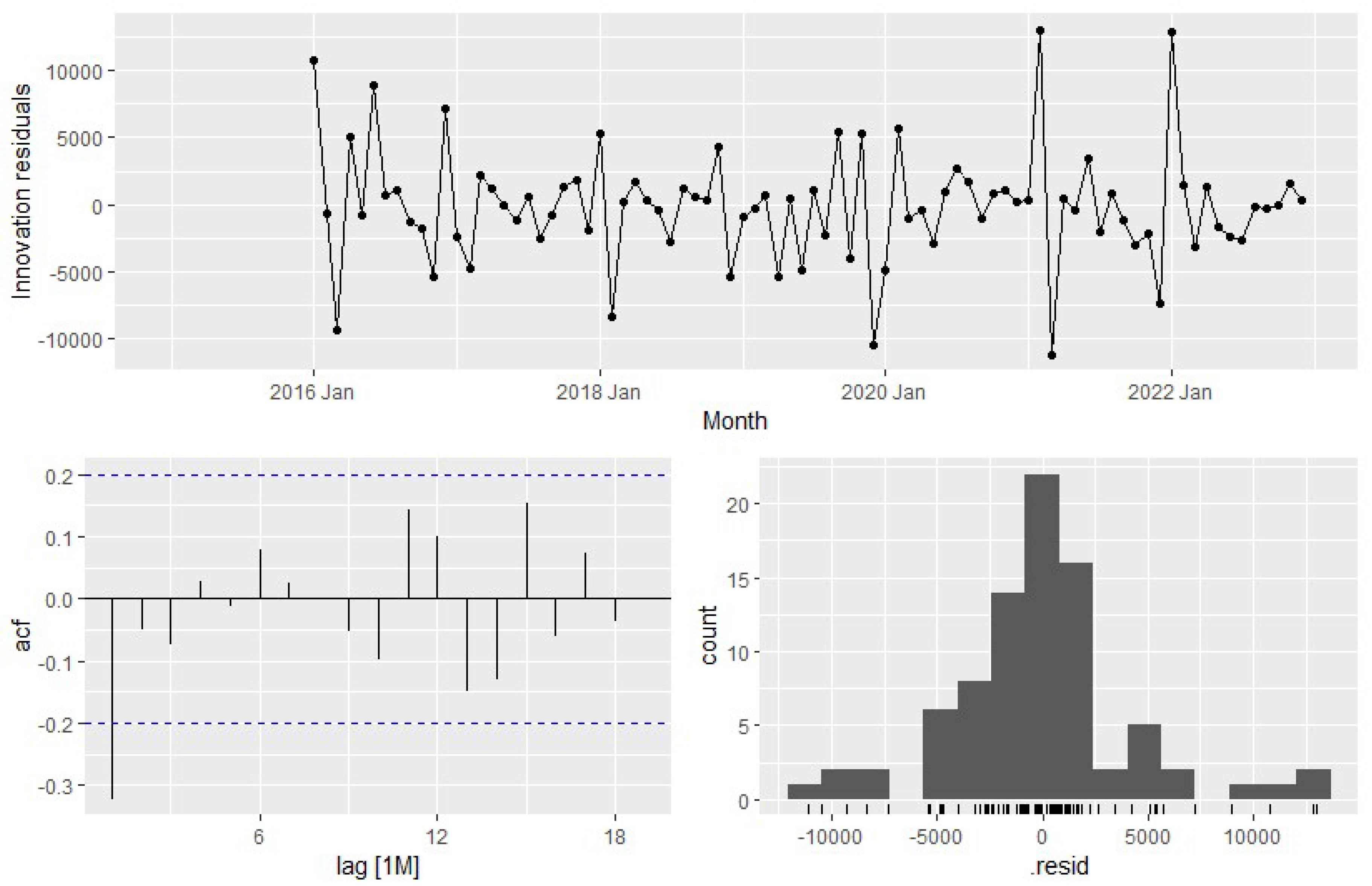
Figure 17.
Residual analysis of SNAÏVE forecasting method.
Figure 17.
Residual analysis of SNAÏVE forecasting method.
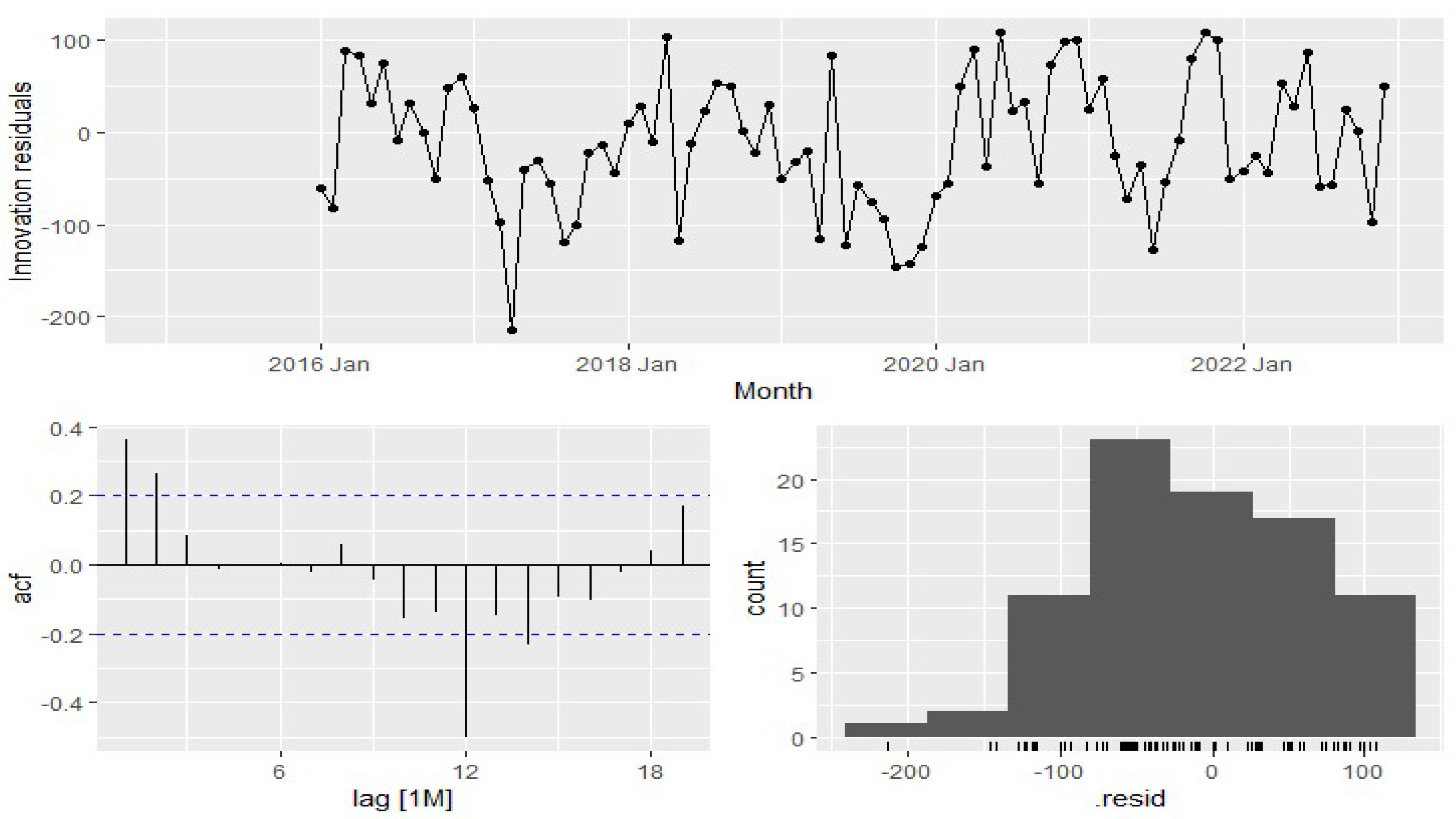
Figure 18.
Residual analysis of ARIMA forecasting method.
Figure 18.
Residual analysis of ARIMA forecasting method.
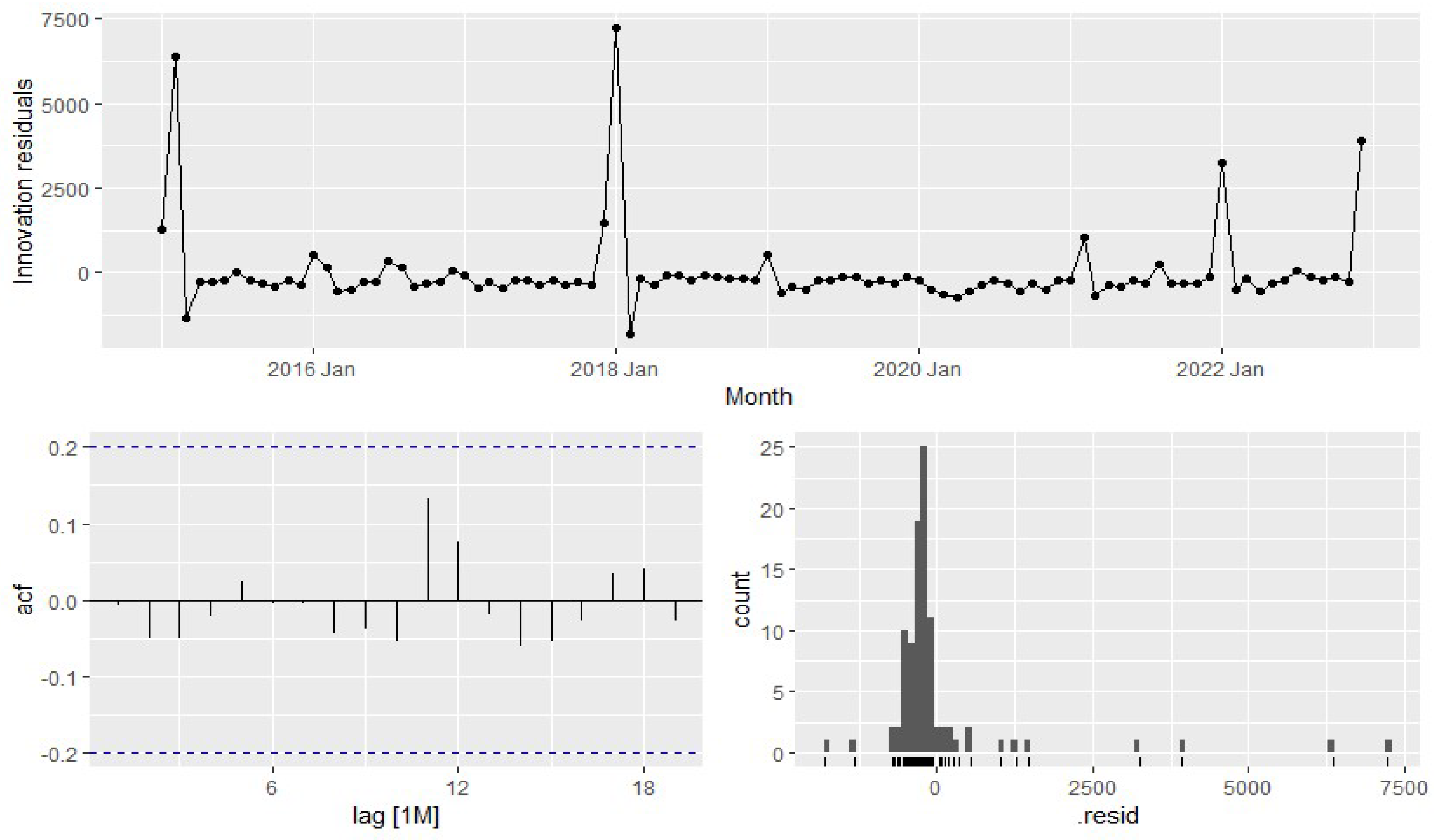
Figure 19.
Overall trend analysis of NG consumption for U.S. electricity generation.
Figure 19.
Overall trend analysis of NG consumption for U.S. electricity generation.
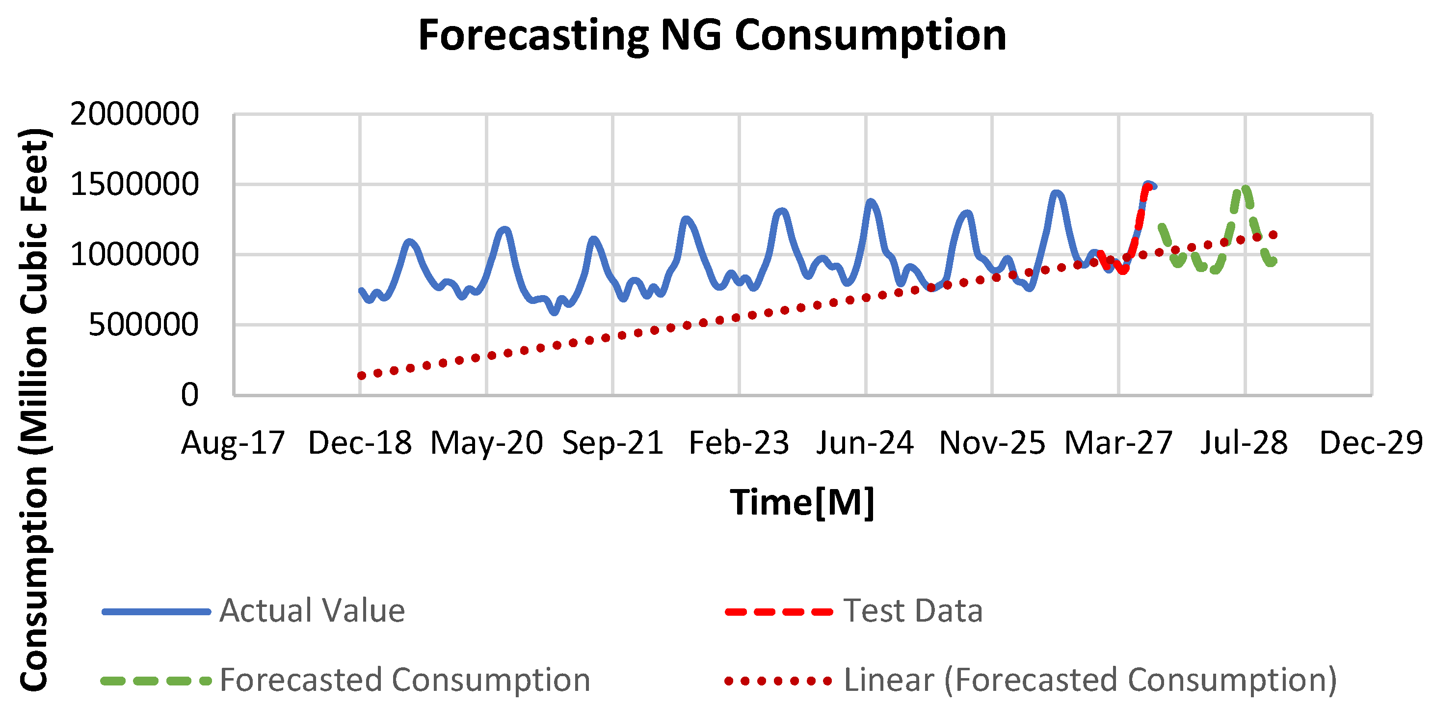
Figure 20.
Overall trend analysis of coal consumption for U.S. electricity generation.
Figure 20.
Overall trend analysis of coal consumption for U.S. electricity generation.
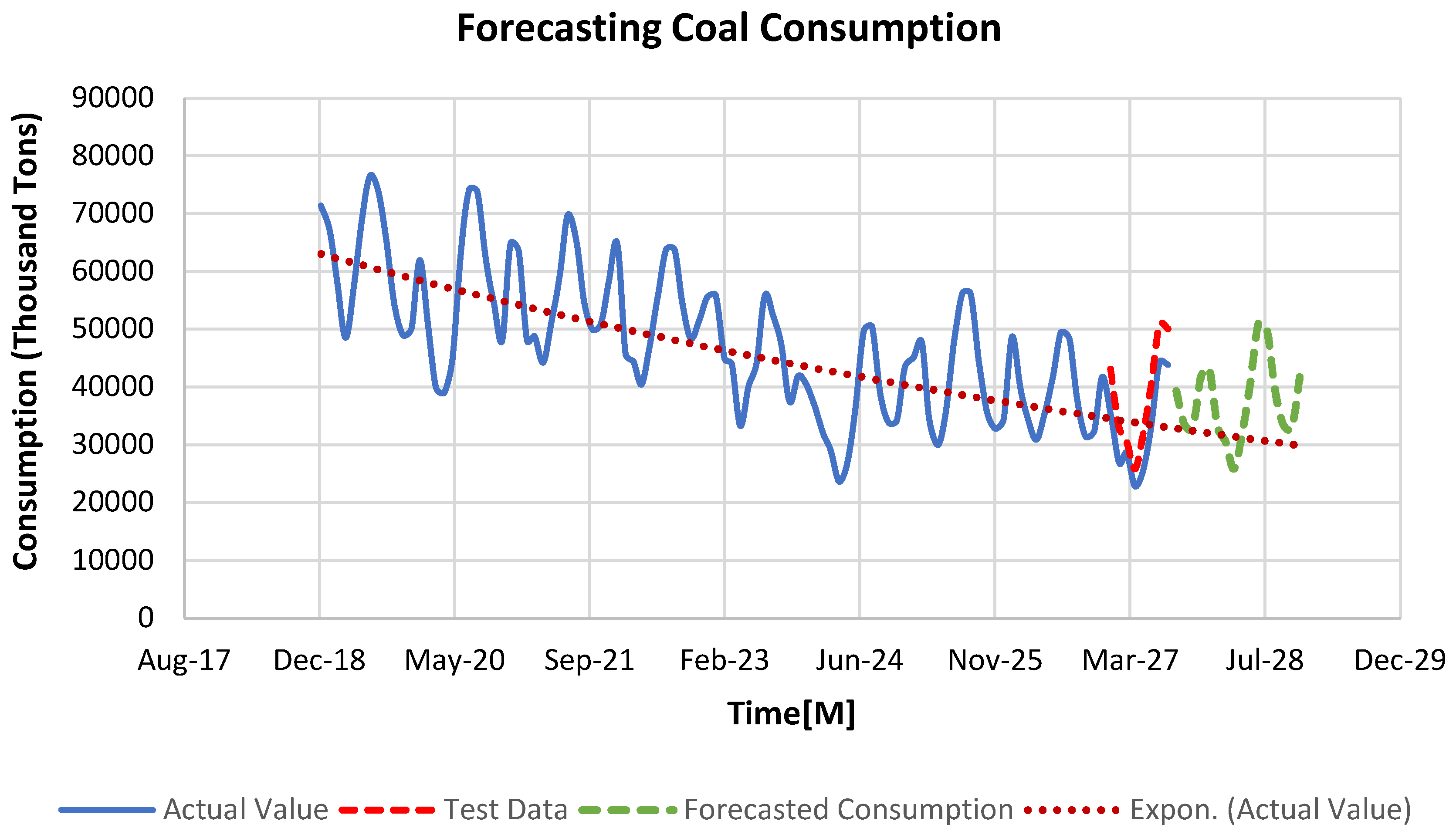
Figure 21.
Overall trend analysis of petroleum coke consumption for U.S. electricity generation.
Figure 21.
Overall trend analysis of petroleum coke consumption for U.S. electricity generation.
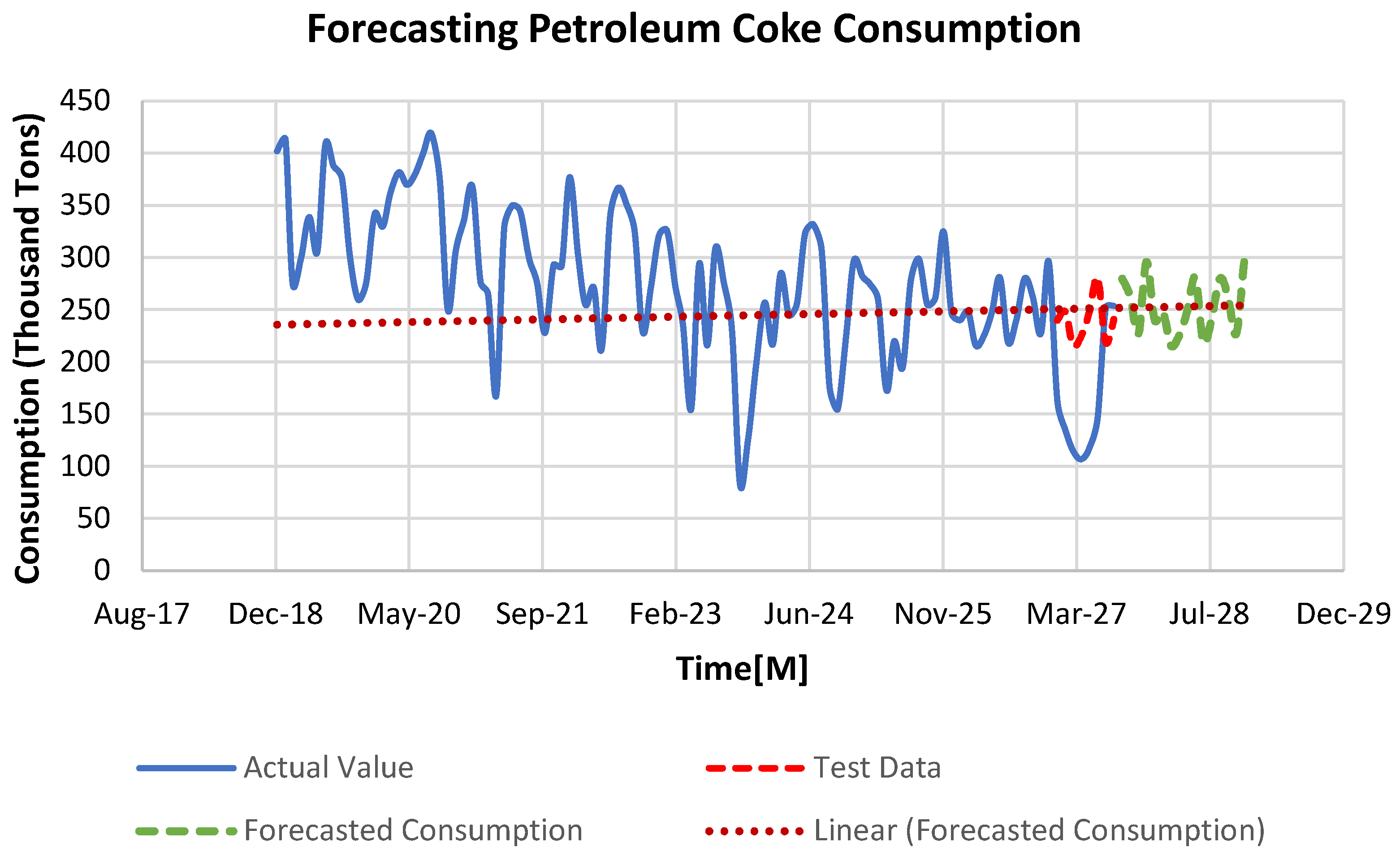
Figure 22.
Overall trend analysis of petroleum liquid consumption for U.S. electricity generation.
Figure 22.
Overall trend analysis of petroleum liquid consumption for U.S. electricity generation.
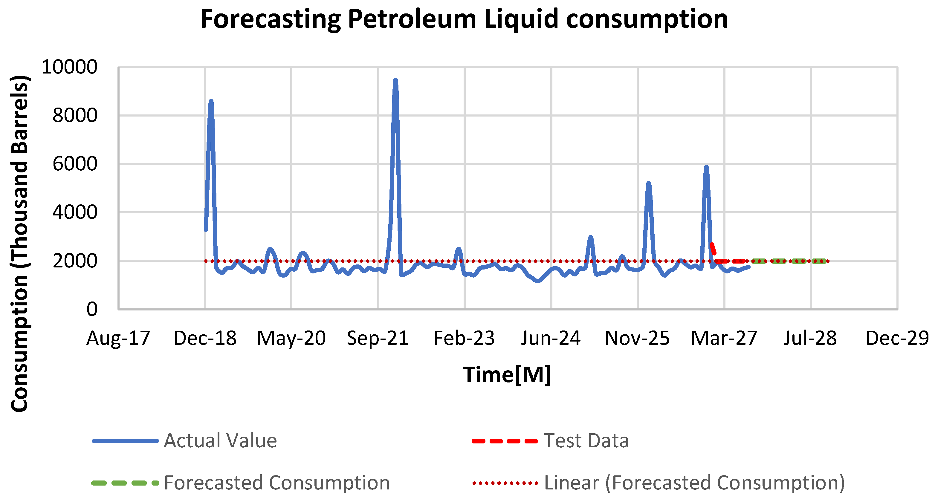
Figure 23.
Forecasted trend of all four components used for fuel consumption to generate electricity.
Figure 23.
Forecasted trend of all four components used for fuel consumption to generate electricity.
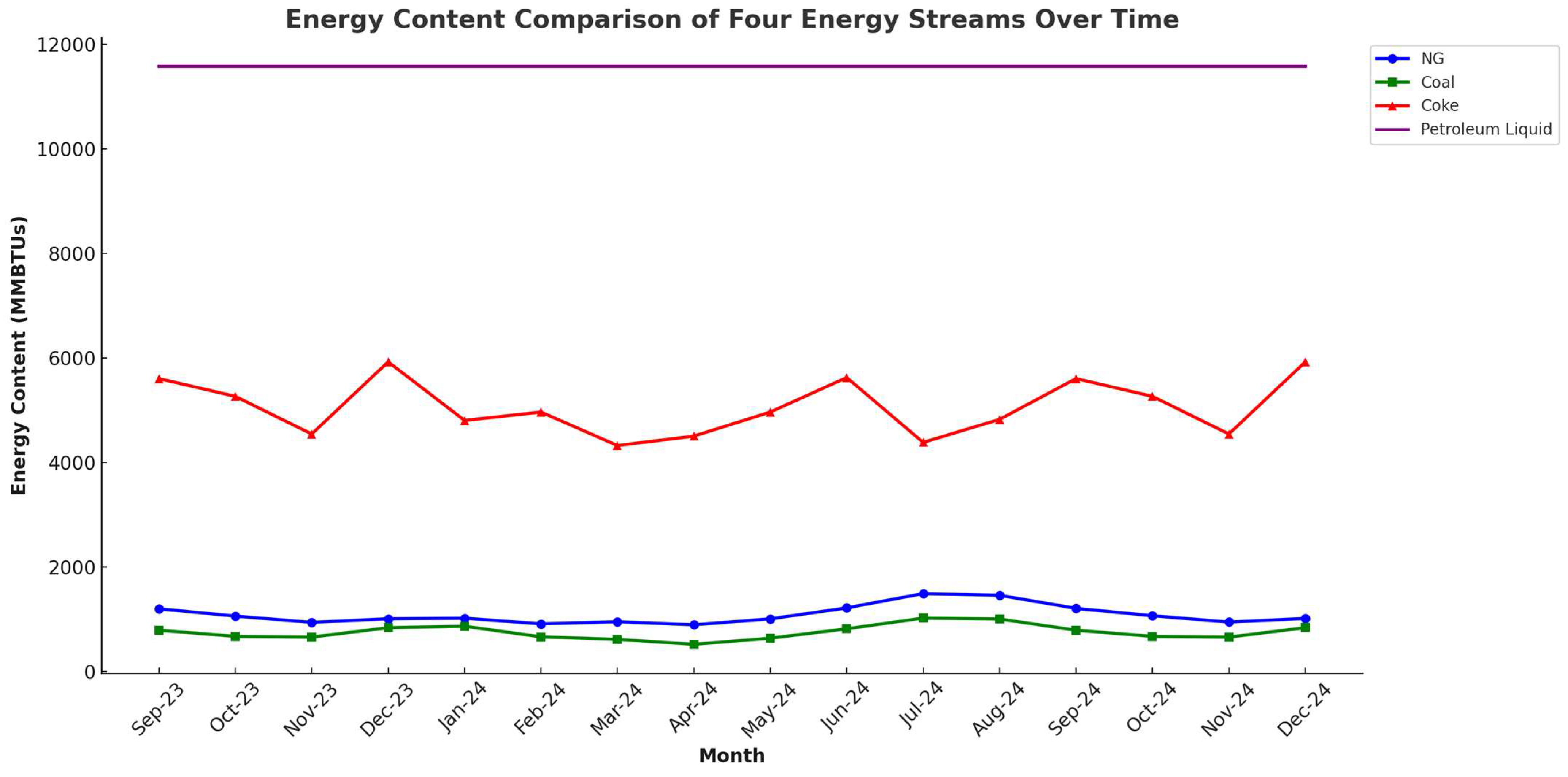
Table 1.
Model comparison in terms of errors for training dataset (NG).
Table 1.
Model comparison in terms of errors for training dataset (NG).
| Training Data | Model | ME | RMSE | MAE | MPE | MAPE | ACF1 |
| STLF | 2485.022 | 46,311.86 | 37,269.12 | 0.19733 | 4.054975 | −0.31132 | |
| ARIMA | −1003.74 | 42,482.11 | 34,075.3 | −0.43476 | 3.772431 | 0.028523 | |
| ETS | 2776.487 | 39,237.5 | 32,580.19 | 0.124194 | 3.633987 | 0.029872 | |
| MEAN | −3.88 × 10⁻¹¹ | 187,831.5 | 150,235 | −3.91587 | 16.47926 | 0.758566 | |
| NAÏVE | 2849.021 | 129,627.5 | 104,644.3 | −0.54117 | 11.12082 | 0.372243 | |
| SNAÏVE | 28,184.8 | 85,297.44 | 72,281.51 | 2.45759 | 8.001223 | 0.716488 | |
| RW-DRIFT | 2.94 × 10⁻¹¹ | 129,596.2 | 104,914.3 | −0.86377 | 11.16892 | 0.372243 |
Table 2.
Model comparison in terms of errors for testing dataset (NG).
Table 2.
Model comparison in terms of errors for testing dataset (NG).
| Testing Data | Model | ME | RMSE | MAE | MPE | MAPE | ACF1 |
| STLF | 14,741.56 | 50,661.2 | 44,064.48 | 0.566659 | 3.729218 | 0.648806 | |
| ARIMA | 25,348.86 | 51,424.27 | 46,082.33 | 1.857718 | 4.030831 | 0.341779 | |
| ETS | 7600.542 | 20,687.46 | 17,204.31 | 0.513017 | 1.477106 | 0.117672 | |
| MEAN | 199,798.9 | 308,728.4 | 212,774.1 | 14.57299 | 16.03116 | 0.650277 | |
| NAÏVE | 99,858.38 | 255,666.4 | 185,054.6 | 5.251944 | 14.63274 | 0.650277 | |
| SNAÏVE | 75,924.13 | 86,594.7 | 75,924.13 | 7.302419 | 7.302419 | 0.271527 | |
| RW-DRIFT | 87,037.78 | 245,731.8 | 181,637.9 | 4.152805 | 14.53365 | 0.647994 |
Table 3.
Model comparison in terms of errors for training dataset (Coal).
Table 3.
Model comparison in terms of errors for training dataset (Coal).
| Training Data | Model | ME | RMSE | MAE | MPE | MAPE | ACF1 |
| STLF | −96.8973 | 4234.149 | 2884.178 | −0.74241 | 6.481808 | −0.32284 | |
| ARIMA | −399.02 | 4385.426 | 3269.713 | −1.15739 | 7.247969 | 0.012544 | |
| ETS | −334.795 | 3831.801 | 2944.868 | −1.1289 | 6.287089 | 0.036044 | |
| MEAN | 2.43 × 10⁻¹² | 12,092.34 | 9731.963 | −6.69494 | 21.85658 | 0.762233 | |
| NAÏVE | −311.937 | 8018.467 | 6701.453 | −1.98137 | 14.30493 | 0.269363 | |
| SNAÏVE | −3190.68 | 7797.248 | 6340.655 | −8.10497 | 14.95868 | 0.679204 | |
| RW-DRIFT | 9.19 × 10⁻¹³ | 8012.397 | 6687.139 | −1.29341 | 14.23191 | 0.269363 |
Table 4.
Model comparison in terms of errors for the testing dataset (Coal).
Table 4.
Model comparison in terms of errors for the testing dataset (Coal).
| Testing Data | Model | ME | RMSE | MAE | MPE | MAPE | ACF1 |
| STLF | −5630.45 | 5936.203 | 5630.449 | −17.4302 | 17.4302 | 0.35842 | |
| ARIMA | −10,728.1 | 11,186.03 | 10,728.1 | −35.0688 | 35.06884 | 0.030943 | |
| ETS | −6864.8 | 7288.344 | 6864.795 | −21.1329 | 21.13289 | 0.338486 | |
| MEAN | −15,923.6 | 17,662.76 | 15,923.57 | −56.8521 | 56.85209 | 0.536813 | |
| NAÏVE | −9111 | 11,892.15 | 10,296 | −34.8482 | 37.53244 | 0.536813 | |
| SNAÏVE | −8444.63 | 9014.585 | 8444.625 | −28.1565 | 28.15649 | 0.300924 | |
| RW-DRIFT | −7707.28 | 11,166.73 | 10,062.05 | −30.5693 | 35.90604 | 0.560167 |
Table 5.
Model comparison in terms of errors for training dataset (Coak).
Table 5.
Model comparison in terms of errors for training dataset (Coak).
| Training Data | Model | ME | RMSE | MAE | MPE | MAPE | ACF1 |
| STLF | 0.072135 | 50.30918 | 38.44801 | −1.7798 | 15.68808 | −0.31094 | |
| ARIMA | −7.79429 | 50.97813 | 39.21442 | −6.92597 | 16.82244 | −0.04866 | |
| ETS | −2.2064 | 44.60708 | 35.05145 | −3.58674 | 14.38404 | 0.147046 | |
| MEAN | 0 | 66.17165 | 52.33333 | −7.38547 | 21.85282 | 0.57797 | |
| NAÏVE | −1.11579 | 59.88902 | 47.55789 | −3.72212 | 19.53299 | −0.17484 | |
| SNAÏVE | −12.619 | 71.87241 | 60.09524 | −9.37567 | 25.92356 | 0.360049 | |
| RW-DRIFT | 1.08 × 10⁻¹⁴ | 59.87863 | 47.54859 | −3.2987 | 19.48854 | −0.17484 |
Table 6.
Model comparison in terms of errors for testing dataset (Coak).
Table 6.
Model comparison in terms of errors for testing dataset (Coak).
| Testing Data | Model | ME | RMSE | MAE | MPE | MAPE | ACF1 |
| STLF | −134.524 | 139.2002 | 134.5243 | −97.8964 | 97.89637 | 0.392624 | |
| ARIMA | −100.747 | 115.8635 | 100.7467 | −79.5287 | 79.52873 | 0.571681 | |
| ETS | −130.006 | 134.3647 | 130.0063 | −94.2535 | 94.25347 | 0.375933 | |
| MEAN | −122.75 | 134.7748 | 122.75 | −94.6778 | 94.67779 | 0.558346 | |
| NAÏVE | −134.75 | 145.7884 | 134.75 | −102.904 | 102.9036 | 0.558346 | |
| SNAIVE | −78.5 | 99.49749 | 90 | −64.2448 | 68.79813 | 0.355008 | |
| RW-DRIFT | −129.729 | 141.8381 | 129.7289 | −99.7341 | 99.73414 | 0.565986 |
Table 7.
Model comparison in terms of errors for training dataset (Petroleum Liquids).
Table 7.
Model comparison in terms of errors for training dataset (Petroleum Liquids).
| Training Data | Model | ME | RMSE | MAE | MPE | MAPE | ACF1 |
| STLF | 51.27077 | 1206.734 | 469.8335 | −5.79073 | 20.42126 | −0.351 | |
| ARIMA | −0.39939 | 1199.579 | 556.5674 | −12.6417 | 22.80608 | −0.00636 | |
| ETS | −72.5277 | 1522.814 | 687.7297 | −11.0457 | 34.25543 | −0.26354 | |
| MEAN | 0 | 1214.503 | 563.3268 | −12.923 | 23.11294 | 0.136773 | |
| NAÏVE | 27.18947 | 1548.012 | 604.3474 | −9.65595 | 25.94808 | −0.37293 | |
| SNAÏVE | −1.96429 | 1494.727 | 578.4881 | −6.82803 | 22.23511 | 0.142605 | |
| RW-DRIFT | −1.82 × 10⁻¹³ | 1547.773 | 604.41 | −11.2077 | 26.08228 | −0.37293 |
Table 8.
Model comparison in terms of errors for testing dataset (Petroleum Liquids.
Table 8.
Model comparison in terms of errors for testing dataset (Petroleum Liquids.
| Testing Data | Model | ME | RMSE | MAE | MPE | MAPE | ACF1 |
| STLF | −3879.82 | 3893.528 | 3879.82 | −225.717 | 225.7167 | −0.24153 | |
| ARIMA | −353.011 | 424.909 | 354.831 | −20.8028 | 20.8937 | −0.39078 | |
| ETS | −6402.64 | 6769.273 | 6402.639 | −365.768 | 365.7678 | 0.550292 | |
| MEAN | −260.063 | 287.3403 | 263.7344 | −15.588 | 15.77136 | 0.232705 | |
| NAÏVE | −4147.75 | 4149.55 | 4147.75 | −241.594 | 241.5938 | 0.232705 | |
| SNAÏVE | −475.75 | 1221.797 | 544.5 | −26.5977 | 30.84144 | −0.00337 | |
| RW-DRIFT | −4270.1 | 4273.105 | 4270.103 | −248.811 | 248.8107 | 0.476336 |
[ad_2]