Generalised Linear Modelling for Construction Waste Estimation in Residential Projects: Case Study in New Zealand
[ad_1]
1. Introduction
The construction industry is known for generating a substantial amount of waste due to excessive consumption of natural resources beyond what is actually required. Tafesse et al. [1] reported that construction waste poses a significant challenge for approximately 95.71% of ongoing construction projects, as it consists of discarded or surplus materials or products that are incompatible with specifications, damaged, or created as secondary products during the construction process [2]. Waste, as defined by the European Council [3], refers to any substance or object that is discarded or intended to be discarded, regardless of whether it is for disposal or recovery operations. Construction waste can have adverse effects on the environment, economy, and social aspects of the industry [4]. Tafesse et al. [1] highlight that globally, construction waste generation leads to cost overruns, environmental pollution, reduced profits, bankrupt construction firms, excessive consumption of raw materials, and risks to public health and safety. Despite the potential for minimising construction waste through practices such as reduction, reuse, and recycling, there is a prevailing tendency among practitioners and workers to dispose of waste in landfills [5]. However, if this trend continues, landfills may soon become inadequate to meet the growing demand. Despite the negative consequences of inadequate waste management, the construction industry has not given sufficient attention to effectively managing construction waste. A large body of recent literature underscores the critical importance of construction minimisation across the project lifecycle, from design and material procurement to construction activities [6,7,8,9]. While various waste reduction solutions exist for all stages of the building process, previous studies have highlighted the significance of taking measures at the early stages in the project lifecycle to effectively manage construction waste [7,10,11,12]. Among these measures, the quantification and prediction of construction waste emerge as pivotal, as they enable industry stakeholders to take appropriate actions at the right time, thereby minimising and managing the generation of construction waste effectively.
2. Construction Waste Prediction and Quantification
Quantifying and predicting construction waste materials in the initial stages of a project are commonly used methods for effective waste management. Around the world, various studies have been conducted to investigate these approaches. To gain a comprehensive understanding of the existing research on methods for quantifying and predicting construction waste, a thorough semi-systematic literature review was performed using the Scopus database. The aim of this literature review was to identify and analyse previous studies related to the quantification and prediction of construction waste materials. By delving into the Scopus database, researchers were able to uncover a total of twenty-eight studies that specifically focused on early quantification and prediction methods for construction waste materials. These studies provide valuable insights into the methods and strategies employed in assessing and forecasting construction waste at the early stages of a project. Figure 1 illustrates the main methods used for early quantification/prediction, which can be categorised into five distinct groups: waste generation rate (WGR) method, variables modelling (VM) method, bill of quantity-based classification system (BoQs) method, BIM-based classification system (BIMS) method, and other methods. These studies utilised direct measurements on site, indirect measurements, secondary data, and user inputs to quantify and predict construction waste generation.
The WGR method involves calculating the waste generation rate (WGR) per unit of construction area. By multiplying the WGR by the total construction area, the total construction waste can be easily determined [13] Some authors have applied this method to calculate waste generation rates for specific material types, such as concrete, steel, wood, masonry, and tiles [14,15]. While the WGR method allows for the development of site waste management plans, a limitation is the inability to track the origin of waste from specific construction activities and elements, thereby impeding source waste reduction efforts.
The variable modelling method is frequently employed to predict waste generation based on project characteristics. This method provides more accurate results in the early stages of a project compared to the WGR method as it considers variables beyond construction area that influence waste generation, such as structural types, design parameters, and economic indicators. Multiple linear regression analysis is commonly utilised to establish the relationship between predictor variables and waste generation [4,11,13,16,17]. Furthermore, Maués et al. [18] developed a fuzzy logic model, and artificial intelligence data-driven methods have been employed to predict waste quantities by capturing complex non-linear relationships using historical data [19,20,21].
Waste estimation based on the bill of quantity (BoQ) classification system is another commonly used method. In this approach, the total waste is determined by summing the waste quantities of all items listed in the BoQ. The BoQs method estimates waste quantities based on project design, incorporates waste categorisation by material type, and enables waste source tracking. However, this method relies on the availability of the bill of quantities, thereby limiting waste assessment during the early design stage. BIM-based waste estimation follows a similar principle as the BoQ method but incorporates the estimation model within Building Information Modelling (BIM) software. This integration allows for automatic waste quantity estimation and updates throughout the design stage. Other waste estimation methods include calculations based on the difference between purchased and required materials [14,22,23] and multiplying the total quantity of consumed material by a transformation coefficient [24].
3. Construction Waste Generation in Residential Projects in New Zealand
In New Zealand (NZ), the construction industry significantly contributes to the overall waste in landfills, accounting for nearly 50% of it [4,25] A survey conducted by the Ministry for the Environment in 2018 ranked waste reduction as the third most significant challenge facing New Zealanders in the next two decades. In this context, residential construction waste reduction holds paramount significance, particularly given that approximately 70% of the country’s construction activities are attributed to residential building projects, as reported by Stats NZ [26]. The demand for residential construction activities has been consistently high, leading to an annual increase of approximately 7–8% in the issuance of new consents [27]. In light of the “net zero waste” objective set to be achieved by 2040, the New Zealand residential construction sector plays a critical role in the country’s waste reduction efforts. Statistical data reveals that New Zealand industries and households dispose of more than 3 million tonnes of construction and demolition debris into landfills and clean fills every year, averaging about one tonne per person [28].
Numerous researchers worldwide have conducted studies specifically targeting the reduction of construction waste in residential projects. Sáez, del Río Merino, Porras-Amores, and González [29] conducted research specifically focused on residential projects and found that the intermediate phases of a project significantly contribute to waste generation. They were able to determine that the weight of waste per floor area amounts to 117.5 kg/m2 (or 0.18 m3/m2 in volume). A study by Mahayuddian et al. [30] identified the average waste generation rate (WGR) in residential buildings in Malaysia as 16.6 kg/m2. Similarly, Saez et al. (2014) [31] reported a figure of 21.4 kg/m2 in Spain. Moreover, Domingo and Batty [4] revealed that the waste generation rate per gross floor area (WGR) of residential projects in New Zealand stands at 32.2 kg/m2, placing it in the mid-range when compared internationally.
Accurate waste prediction information plays a vital role in establishing a robust foundation for waste recycling and utilisation, which are of utmost importance [32]. Predicting construction waste quantities, as part of the project execution plan, is crucial for effective project planning and execution. In the methods outlined in Section 2, waste generation rate (WGR) and variable modelling techniques are the applicable means for estimating and predicting waste generation during the initial phases of a construction project with minimal information. In comparison to the WGR method, variable modelling holds greater potential for aiding design teams in making informed decisions regarding waste source reduction through the optimisation of design parameters in a building. However, developing a precise method for waste estimation and prediction is challenging, as the results heavily rely on geographical, technical, and cultural variables [33]. The available waste-related ratios and models are subjective, as they heavily depend on parameters such as building type, construction methodology, construction materials, and the construction region or country. Saez [31] emphasised that adopting waste quantities from other regions or construction methods can lead to inaccurate results.
Similarly, Domingo and Batty [4] emphasised the distinctive nature of the New Zealand construction industry, characterised by variations in materials, especially timber framing and structures, technologies, and processes. Owing to methodological disparities in construction practices across different countries, adopting existing models to predict waste generation in diverse contexts proves challenging. Consequently, this study focuses on developing an accurate construction waste prediction model specifically tailored for residential projects in New Zealand, utilising design parameters as the foundation for estimation.
4. Methodology
To accomplish the aforementioned research objective of developing a model for estimating construction waste during the early design stage of residential construction projects, a quantitative approach was employed in this study. A total of 213 detached residential projects were utilised, and both waste quantities and building designs were taken into consideration. These projects were systematically selected to represent the typical range of construction styles and sizes observed in New Zealand, encompassing the work of several small builders. The sample spanned a period of approximately seven years, from 2015 to 2023. Within the sample, there were residential projects completed by a national builder (n = 162) as well as several small builders located in Palmerston North and Manawatu (n = 51) in New Zealand. A smaller subset of the sample comprised architectural-style homes. The selected projects predominantly featured detached houses with raft slab foundations, pre-nail timber frames, colour steel roofing, and board/sheet and brick or stone cladding. The data collected for analysis were divided into response variables and predictor variables.
4.1. Response Variable
The response variable utilised in this study was the waste volume of each residential building. The waste volume for each building was determined by calculating a summary of the waste data provided by the waste collection company, which was based on the number of skips used and the weights recorded at the dumpsite. The waste data were typically rounded to the nearest 250 or 500 kg and expressed in tonnes, reflecting the measurable quantity of a skip bin. The waste volumes observed in the construction of New Zealand residential buildings exhibited a highly positively skewed distribution, with a median value of 6.20 tonnes. There were a few buildings that exhibited higher waste volumes, reaching up to 15.00 tonnes (refer to Figure 2 and Table 1). As there were no miscalculations or significant differences in the architectural aspects, the houses with greater waste volumes (>10 tonnes) were included in the analysis, as they were assumed to contribute to the inherent variation in waste volume generated by housing projects. Additionally, a Mann–Whitney U test provided strong evidence (W = 1570.5, p value = 2.56 × 10⁻¹¹; see Supplementary Figure 2 indicating that waste volumes were significantly greater in single-family houses constructed by Palmerston North and Manawatu builders (subset2, median = 7.25 tonnes) compared to those built by the national builder (subset1, median = 5.43 tonnes).
4.2. Predictor Variables
The predictor variables for this study were chosen based on the methods outlined by Domingo and Batty [4], considering their impact on construction cost and material input. A total of nine numerical variables (refer to Table 1) and four categorical variables (refer to Table 2) were employed as predictor variables in the statistical models utilised in this study. Design measurements such as floor area, internal wall length, external perimeter, roof area, cladding types and areas, number of corners, number of stories, and number of bathrooms were extracted from architectural plans as well as tracked during the construction process. In cases where architectural plans were not available, on-site physical measurements were conducted to collect the necessary data. However, it should be noted that roof area and roof cladding type were only accessible for houses within subset 2 of the sample. The number of working days was calculated by adjusting the project duration to account for statutory holidays, Christmas shutdown periods, and COVID-19 lockdown periods.
The sample consisted of two types of detached houses: single-family houses and houses with a self-contained flat/granny flat/rental unit. The houses included in the analysis comprised both one-storey and two-storey structures. However, one house with 1.5 stories and two houses with 1.5 and 5 bathrooms, respectively, were excluded from the analysis due to the small sample sizes for these specific levels compared to the other levels within their respective categories (see Table 2). Additionally, similar to the waste volume, certain variables such as floor area, working days, external perimeter, internal wall length, roof area, and different cladding areas (board, sheet, and brick or stone) indicated that there were a few buildings with larger built areas compared to the majority of residential buildings (see Table 1). However, upon closer examination, no discernible patterns were observed among residential buildings with higher waste volumes (>10 tonnes) and larger built areas. Consequently, it was assumed that houses with greater built areas also contributed to the natural variation in the built area of housing projects in New Zealand.
5. Results
Multiple generalised linear models were fitted to develop a tool that predicts the waste volume of residential buildings with the highest accuracy. This involved two approaches: (a) combining predictor variables additively in different combinations, and (b) using different subsets of data. To identify highly correlated parameters, a Pearson correlation analysis was initially conducted. The results of this analysis are illustrated in Figure 3.
5.1. Predicting Waste Volume without Roof Parameters
The correlation analysis revealed a strong correlation of 0.96 between floor area and roof area. Consequently, roof parameters were excluded from the initial model. The dataset was divided into training (n = 160) and test (n = 50) sets using the ‘sample.split()’ function from the ‘caTools’ package [34] in the R statistical software, version 4.2.0 [35]. Generalised linear models were fitted for waste volume using both subset1 and subset2 together to investigate the impact of design parameters, project timeline, and builder type on waste volume. The ‘glm()’ function from the ‘stats’ package [36] was employed for model fitting. The Akaike information criterion (AIC) was used as a measure to evaluate model fitness. The model with the lowest AIC value, determined through the ‘stepAIC()’ function in the ‘MASS’ package [37,38], was selected as the best-fitting model. The stepwise procedure started with the full model and iteratively removed one variable at a time while adding another variable to obtain different combinations of predictor variables, aiming for the optimal fit with the lowest AIC. The models were evaluated based on their statistical properties using AIC values, and the accuracy of prediction was assessed using the test data for the prediction tool. The ‘predict()’ function in the ‘car’ package [39] was employed to calculate the model predictions and determine the 99% confidence interval of the predictions. The best prediction model, excluding roof parameters, was chosen based on its lower AIC value and the highest prediction accuracy on the test dataset. A prediction was considered accurate if the actual waste volume fell within the predicted 99% confidence interval.
5.2. Predicting Waste Volume with Roof Parameters
In the second attempt, the prediction tool was enhanced by including roof parameters, as suggested by the existing literature, which indicates that roofing systems contribute more to construction waste compared to floors or walls, primarily due to their complexity [40]. Subset2 was utilised for model fitting, and since roof area exhibited a strong correlation with floor area, internal wall length, and external perimeter (correlation coefficient > 0.7), the number of variables was reduced to orthogonal axes using principal component analysis (PCA). This approach allowed for a generalised representation of the built area through the extracted principal components. The data were subsequently divided into training (n = 43) and test (n = 8) sets, and models were trained using the training data. Different combinations of predictor variables were employed as fixed effects in the model training process. The model with the lowest AIC value and the highest prediction accuracy on the test dataset was identified as the best prediction model incorporating roof parameters.
5.3. Prediction Tool
To reduce the generalization error of prediction, the prediction tool was developed using ensemble models [41]. The models with the highest accuracy for predicting the waste volumes with and without roof parameters were used in the prediction tool. Here, estimated waste volumes from both models (with and without roof parameters) were averaged to deliver the final prediction with a 99% confidence interval.
5.4. Predicting Waste Volume without Roof Parameters
The best-fitting model (model 1) to describe the waste volume with the lowest AIC (516.28) contained the number of working days, corners, floor area and the builder type as fixed factors. The number of working days, corners, and floor area showed a strong positive correlation with the waste volume (Table 3; p value Table 3; p value
Since the accuracy of the predictions was low in model 1, the model was extended by adding other predictor variables, as shown in Table 2.
The model with highest accuracy in predictions (model 2: 80.00% accuracy), with an AIC of 528.25, showed that having all predictor variables increased the accuracy of the predictions (Table 4). In addition to the positive correlation between working days, floor area, and number of corners as in model 1, model 2 showed that having two complete bathrooms and a powder-room/toilet increased the waste volume compared to having one bathroom. Comparing the fitness of model 2 with model 1, using the ‘lrtest’ function in the ‘lmtest’ package, revealed that the fitness of model 2 was not significantly different to model 1 (chisq = 12.03, p value > 0.05). Therefore, model 2 can be used as the prediction model without roof parameters.
5.5. Predicting Waste Volume with Roof Parameters
Two principal components were extracted from the principal component analysis (Table 5). All four parameters contributed to the first principal component (PC1), which explained 89.93% of the total variance (eigenvalue = 3.57); and internal wall length and roof area contributed to the second principal component (PC2), which explained 7.41% of the total variance (eigenvalue = 0.30). Together, PC1 and PC2 explained 97.34% of the total variance (Table 6). The best-fitting model (model 3) with roof parameters to describe the waste volume with the lowest AIC (71.48) contained the number of stories, sheet cladding area, PC1, and PC2 as the fixed factors of the model. The accuracy of the predicted values for model 3 was 75.00% for the test data. In model 3, there was strong evidence that PC1 and PC2 showed a negative correlation with the waste volume (Table 7; p value
However, when model 3 was extended by adding other predictor variables (see all models in Table 6) the model with the highest accuracy in predictions (model 4), with an AIC of 76.07, showed that addition of roof cladding type, the number of working days, and bathrooms increased the accuracy of predictions in the test data to 100.00% (Table 6). Similar to model 3, model 4 also showed strong evidence that PC1 (overall built area) had a positive correlation with the waste volume (Table 7; p p value > 0.05) as shown in Table 8. Therefore, model 4 can be used as the prediction model with roof parameters.
5.6. Prediction Tool
Finally, ensemble models (model 2 and model 4) were used to calculate the final prediction and 99% confidence intervals for the prediction using the test data (n = 8) of subset 2. The tool demonstrated that 100% of the actual waste volumes were within the predicted range (Table 9).
6. Discussion
In the literature, there are several variable modelling techniques available to measure and predict construction waste generation using different approaches. For instance, Hu et al. [19] employed design features such as floor area, height, and material quantities that go into different building components to estimate construction waste generation on site. This model significantly contributes to enabling construction teams to predict and manage construction waste generation in materials. However, a more detailed level of design is required to apply this model to material waste prediction. Islam et al. [16] followed a rigorous approach to waste prediction, using regression analysis to predict construction and demolition waste based on the estimation of total floor area and waste generation rate. However, this method does not support design teams in making informed decisions on design parameters and waste generation. Domingo and Batty [4] and Keren et al. [11] identified a comprehensive relationship between building waste and building characteristics. Both studies used multiple regression analysis to develop waste prediction models with various design parameters. However, the accuracy of these models ranges between 60 and 70%, leaving room for further improvement to increase the accuracy.
Multiple regression models assume the distribution of the response variable is normal, while generalised linear models (GLMs) allow for a more flexible approximation of the response variable distribution, including non-normal distributions such as gamma or Poisson distributions [42]. Positively skewed response variables, such as the amount of waste generated in residential construction projects (Figure 2), can be better described by GLMs than multiple regression models. This is because multiple regression models assume a symmetric distribution, which may not accurately capture the shape of a positively skewed distribution. Generalised linear models can accommodate positively skewed distributions by allowing for different types of link functions, such as log-link functions, which can transform the response variable to better approximate a normal distribution. Therefore, GLMs used in this study can better capture the underlying distributional properties of the building and project data, leading to more accurate and reliable statistical inference than the models used in Domingo and Batty [4].
This article presents a comprehensive investigation into the residential building design factors influencing construction waste volume, utilising multiple predictive models. The study primarily focuses on identifying the best-fit model to enhance the accuracy of waste volume predictions. As the Pearson correlation analysis shows a strong correlation between floor area and roof parameters, the analysis involves three distinct models (model 2, model 3, and model 4), each incorporating different sets of predictor variables. The findings reveal intriguing insights into the correlation between various construction parameters and waste generation.
The increasing importance of sustainable construction practices has spurred research into understanding and predicting construction waste volume. This study delves into three predictive models, aiming to identify the most influential factors and enhance prediction accuracy. Notably, the research explores the impact of roof parameters on waste generation, shedding light on previously underexplored dimensions of construction waste modelling.
The initial model (model 1) establishes a strong correlation between construction waste volume and fundamental factors such as working days, corners, and floor area. Intriguingly, residential projects led by small builders exhibit significantly higher waste generation, providing valuable insights for waste management strategies. Model 2 introduces enhanced accuracy (80.00%) by incorporating additional predictor variables, notably the presence of multiple bathrooms. Despite the increased accuracy, the study suggests that the fitness of model 2 is not significantly different from model 1, emphasising the practicality of model 2 for prediction without roof parameters. The incorporation of PCA elucidates the dominant factors contributing to waste generation. PC1, representing overall built area, emerges as a significant contributor to waste volume. PC2, influenced by internal wall length and roof area, provides supplementary insights. The combination of PC1 and PC2 explains a substantial 97.34% of the total variance, underscoring their importance in waste volume prediction. Model 3 introduces roof parameters, showing a lower AIC (71.48) and an accuracy of 75.00%. The negative correlation observed between PC1, PC2, and waste volume suggests that reducing the built area may mitigate waste generation. Moreover, the study identifies a positive correlation between adding extra levels to a structure and increased waste volume. The final model (model 4) incorporates roof cladding type, working days, and bathrooms, achieving a remarkable 100.00% accuracy in test data predictions. The positive correlation between PC1 and waste volume is reaffirmed. Importantly, model 4 does not exhibit a significant difference in fitness compared to model 3, signifying its applicability for accurate predictions with roof parameters.
7. Conclusions
This study employed generalised linear models to examine the relationship between design features and waste generation in residential buildings within New Zealand. Generalised linear models were chosen due to their ability to offer a more flexible approximation of the distribution of the response variable, surpassing the capabilities of multiple regression models. Consequently, this approach enabled the development of a model with a high level of accuracy, estimating construction waste generation in residential projects within New Zealand at approximately 80% accuracy.
The analysis revealed that small builders tend to generate a greater amount of waste in residential projects compared to national builders, as supported by compelling evidence obtained from the model. Furthermore, the results indicate that enhancing the accuracy of waste estimation can be achieved by incorporating additional design features into the model. Principal component analysis demonstrated that certain design features, specifically overall built area, internal wall length, and roof area, significantly contributed to the variance in waste volumes. This implies that these particular design aspects exert a substantial influence on waste generation, surpassing the impact of other design features. Additionally, the findings indicate that the overall waste volume can be reduced by minimising the number of bathrooms and the overall built area. The implications of this study’s findings are particularly valuable to construction stakeholders, especially those involved in the design phase, as they offer insights into minimising waste generation by optimising design parameters. By implementing the recommendations derived from this study, construction industry professionals can contribute to sustainable practices and waste reduction in residential projects.
Author Contributions
Conceptualisation, N.D. and R.K.; methodology, N.D., G.W. and H.M.E.; formal analysis, H.M.E. and R.K.; investigation, N.D., H.M.E. and R.K.; resources, N.D.; data curation, N.D., R.K. and H.M.E.; writing—original draft preparation, N.D., H.M.E. and G.W.; writing—review and editing, N.D.; visualisation, N.D., H.M.E. and R.K.; supervision, N.D.; project administration, N.D.; funding acquisition, N.D. All authors have read and agreed to the published version of the manuscript.
Funding
This research was funded by Auckland Council Waste Management and Innovation Fund, grant number WMIF2002-026.
Institutional Review Board Statement
The research project was conducted according to the guidelines of Massey University Human Ethics Committees. The project has been evaluated by peer review and judged to be low risk. Human Ethics Notification–4000024389.
Data Availability Statement
Data available upon request.
Conflicts of Interest
The authors declare no conflict of interest.
References
- Tafesse, S.; Girma, Y.E.; Dessalegn, E. Analysis of the socio-economic and environmental impacts of construction waste and management practices. Heliyon 2022, 8, e09169. [Google Scholar] [CrossRef]
- Skoyles, E.R. Waste Prevention on Site; BT Batsford Limited.: London, UK, 1987. [Google Scholar]
- European Directive 2008/98/EC; Waste Framework Directive Targeting Construction and Demolition Waste and Waste from Households. European Council: Brussels, Belgium, 2008.
- Domingo, N.; Batty, T. Construction waste modelling for residential construction projects in New Zealand to enhance design outcomes. Waste Manag. 2021, 120, 484–493. [Google Scholar] [CrossRef]
- Mah, C.M.; Fujiwara, T.; Ho, C.S. Environmental impacts of construction and demolition waste management alternatives. Chem. Eng. Trans. 2018, 63, 343–348. [Google Scholar]
- Bajjou, M.S.; Chafi, A. Exploring the critical waste factors affecting construction projects. Eng. Constr. Arch. Manag. 2021, 29, 2268–2299. [Google Scholar] [CrossRef]
- Llatas, C.; Osmani, M. Development and validation of a building design waste reduction model. Waste Manag. 2016, 56, 318–336. [Google Scholar] [CrossRef] [PubMed]
- Luangcharoenrat, C.; Intrachooto, S.; Peansupap, V.; Sutthinarakorn, W. Factors Influencing Construction Waste Generation in Building Construction: Thailand’s Perspective. Sustainability 2019, 11, 3638. [Google Scholar] [CrossRef]
- Udawatta, N.; Zuo, J.; Chiveralla, K.; Zillante, G. Improving waste management in construction projects: An Australian study. Resour. Conserv. Recycl. 2015, 101, 73–83. [Google Scholar] [CrossRef]
- Esa, M.R.; Halog, A.; Rigamonti, L. Strategies for minimizing construction and demolition wastes in Malaysia. Resour. Conserv. Recycl. 2017, 120, 219–229. [Google Scholar] [CrossRef]
- Parisi Kern, A.; Dias, M.; Kulakowski, M.P.; Gomas, L.P. Waste generated in high rise buildings construction: A quantification model based on statistical multiple regression. Waste Manag. 2015, 39, 35–44. [Google Scholar] [CrossRef]
- Osmani, M.; Glass, J.; Price, A. Architects’ perspectives on construction waste reduction by design. Waste Manag. 2008, 28, 1147–1158. [Google Scholar] [CrossRef]
- Ripley, B.; Venables, B.; Bates, D.M.; Hornik, K.; Gebhardt, A.; Firth, D.; Ripley, M.B. Package ‘mass’. Cran. R 2013, 538, 113–120. [Google Scholar]
- Bakshan, A.; Srour, I.; Chehab, G.; El-Fadel, M. A field based methodology for estimating waste generation rates at various stages of construction projects. Resour. Conserv. Recycl. 2015, 100, 70–80. [Google Scholar] [CrossRef]
- Li, J.; Ding, Z.; Mi, X.; Wang, J. A model for estimating construction waste generation index for building project in China. Resour. Conserv. Recycl. 2013, 74, 20–26. [Google Scholar] [CrossRef]
- Islam, R.; Nazifa, T.H.; Yuniarto, A.; Uddin, A.S.; Salmiati, S.; Shahid, S. An empirical study of construction and demolition waste generation and implication of recycling. Waste Manag. 2019, 95, 10–21. [Google Scholar] [CrossRef] [PubMed]
- Sáez, P.V.; Porras-Amores, C.; del Río Merino, M. New quantification proposal for construction waste generation in new residential constructions. J. Clean. Prod. 2015, 102, 58–65. [Google Scholar] [CrossRef]
- Maués, L.M.F.; Nascimento, B.D.M.O.D.; Lu, W.; Xue, F. Estimating construction waste generation in residential buildings: A fuzzy set theory approach in the Brazilian Amazon. J. Clean. Prod. 2020, 265, 121779. [Google Scholar] [CrossRef]
- Hu, R.; Chen, K.; Chen, W.; Wang, Q.; Luo, H. Estimation of construction waste generation based on an improved on-site measurement and SVM-based prediction model: A case of commercial buildings in China. Waste Manag. 2021, 126, 791–799. [Google Scholar] [CrossRef] [PubMed]
- Lee, D.; Kim, S.; Kim, S. Development of Hybrid Model for Estimating Construction Waste for Multifamily Residential Buildings Using Artificial Neural Networks and Ant Colony Optimization. Sustainability 2016, 8, 870. [Google Scholar] [CrossRef]
- Liu, J.; Chen, J.; Tang, K. A Method for Estimation of the On-Site Construction Waste Quantity of Residential Projects. In Proceedings of the ICCREM 2018, Charleston, SC, USA, 9–10 August 2018; pp. 225–231. [Google Scholar] [CrossRef]
- Bakchan, A.; Faust, K.M.; Leite, F. Seven-dimensional automated construction waste quantification and management framework: Integration with project and site planning. Resour. Conserv. Recycl. 2019, 146, 462–474. [Google Scholar] [CrossRef]
- Guerra, B.C.; Bakchan, A.; Leite, F.; Faust, K.M. BIM-based automated construction waste estimation algorithms: The case of concrete and drywall waste streams. Waste Manag. 2019, 87, 825–832. [Google Scholar] [CrossRef]
- Mercader-Moyano, P.; Ramírez-De-Arellano-Agudo, A. Selective classification and quantification model of C&D waste from material resources consumed in residential building construction. Waste Manag. Res. 2013, 31, 458–474. [Google Scholar] [CrossRef] [PubMed]
- Ghose, A.; Pizzol, M.; McLaren, S.J. Consequential LCA modelling of building refurbishment in New Zealand- an evaluation of resource and waste management scenarios. J. Clean. Prod. 2017, 165, 119–133. [Google Scholar] [CrossRef]
- Stats NZ. 2024. Available online: https://www.stats.govt.nz/ (accessed on 20 February 2024).
- MBIE. Building and Construction Sector Trends Biannual Snapshot: May 2022. Available online: https://www.mbie.govt.nz/building-and-energy/building/building-system-insights-programme/sector-trends-reporting/biannual-snapshots/november-2022/#:~:text=The%20sector%20had%207%2C035%20more,same%20time%20period%20in%202021 (accessed on 31 January 2024).
- MfE.2023. Waste Generation and Disposal in New Zealand. Available online: https://environment.govt.nz/facts-and-science/waste/waste-facilities-and-disposal/#about-the-data (accessed on 30 September 2023).
- Sáez, P.V.; del Río Merino, M.; Porras-Amores, C.; González, A.S.-A. European Legislation and Implementation Measures in the Management of Construction and Demolition Waste. Open Constr. Build. Technol. J. 2011, 5, 56–161. [Google Scholar]
- Mahayuddin, S.; Pereira, J.J.; Badaruzzaman, W.H.W.; Mokhtar, M.B. Construction Waste Index for Waste Control in Residential House Project. In Proceedings of the SB 10 New Zealand, Te Papa, New Zealand, 26–28 May 2010. [Google Scholar]
- Sáez, P.V.; Merino, M.d.R.; Porras-Amores, C.; González, A.S.-A. Assessing the accumulation of construction waste generation during residential building construction works. Resour. Conserv. Recycl. 2014, 93, 67–74. [Google Scholar] [CrossRef]
- Poon, C.-S.; Yu, A.T.; Jaillon, L. Reducing building waste at construction sites in Hong Kong. Constr. Manag. Econ. 2004, 22, 461–470. [Google Scholar] [CrossRef]
- Nagalli, A. Estimation of construction waste generation using machine learning. Proc. Inst. Civ. Eng.-Waste Resour. Manag. 2021, 174, 22–31. [Google Scholar] [CrossRef]
- Tuszynski, J.; Khachatryan, M.H. Package ‘caTools’. Available online: https://cran.r-project.org/web/packages/caTools/caTools.pdf (accessed on 30 September 2023).
- R Core Team. R: A Language and Environment for Statistical Computing; R Foundation for Statistical Computing: Vienna, Austria, 2022; Available online: http://www.R-project.org (accessed on 31 October 2023).
- Marschner, I.; Donoghoe, M.W.; Donoghoe, M.M.W. Package ‘glm2’. 2018. Available online: https://CRAN.R-project.org/package=glm2 (accessed on 20 February 2024).
- Qiao, L.; Liu, D.; Yuan, X.; Wang, Q.; Ma, Q. Generation and Prediction of Construction and Demolition Waste Using Exponential Smoothing Method: A Case Study of Shandong Province, China. Sustainability 2020, 12, 5094. [Google Scholar] [CrossRef]
- Ripley, B. Choose a Model by AIC in a Stepwise Algorithm; R Doc: Vienna, Austria, 2015. [Google Scholar]
- Fox, J.; Weisberg, S.; Adler, D.; Bates, D.; Baud-Bovy, G.; Ellison, S.; Graves, S. Package ‘car’; R Foundation for Statistical Computing: Vienna, Austria, 2012; p. 16. [Google Scholar]
- Liu, H.; Sydora, C.; Altaf, M.S.; Han, S.; Al-Hussein, M. Towards sustainable construction: BIM-enabled design and planning of roof sheathing installation for prefabricated buildings. J. Clean. Prod. 2019, 235, 1189–1201. [Google Scholar] [CrossRef]
- Kotu, V.; Deshpande, B. Chapter 2—Data Science Process. In Data Science, 2nd ed.; Kotu, V., Deshpande, B., Eds.; Morgan Kaufmann: Burlington, MA, USA, 2019; pp. 19–37. [Google Scholar]
- Dobson, A.J.; Barnett, A.G. An Introduction to Generalized Linear Models, 4th ed.; Chapman and Hall/CRC: Boca Raton, FL, USA, 2018. [Google Scholar] [CrossRef]
Figure 1.
Construction waste estimation methods.
Figure 1.
Construction waste estimation methods.
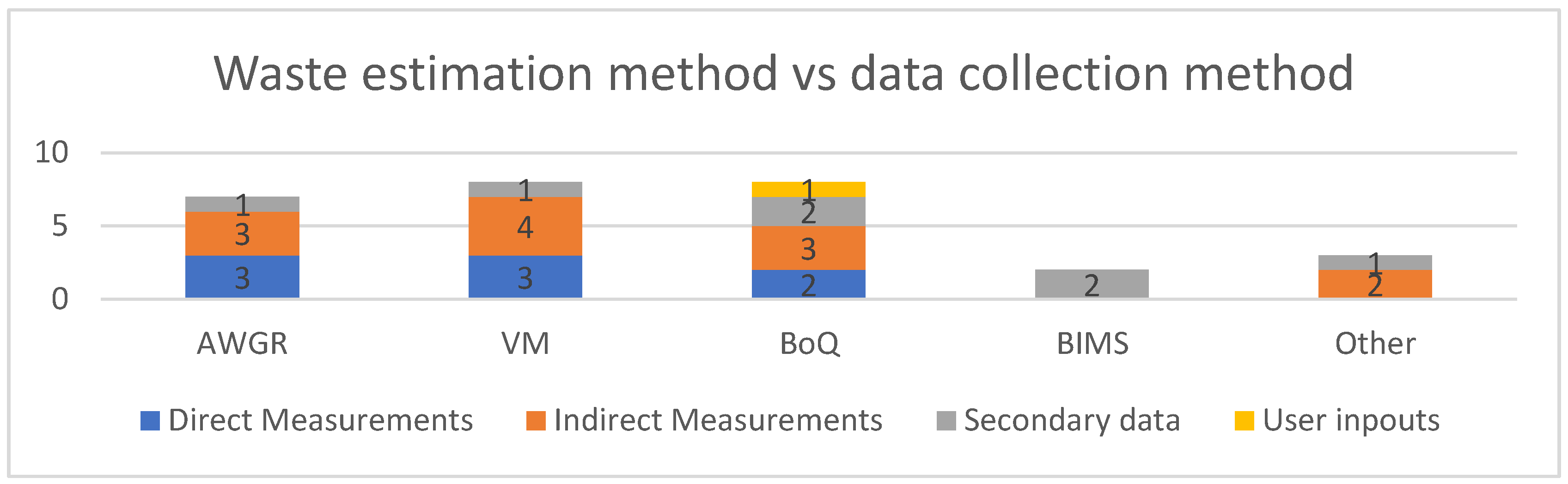
Figure 2.
Waste volume from construction of residential buildings.
Figure 2.
Waste volume from construction of residential buildings.
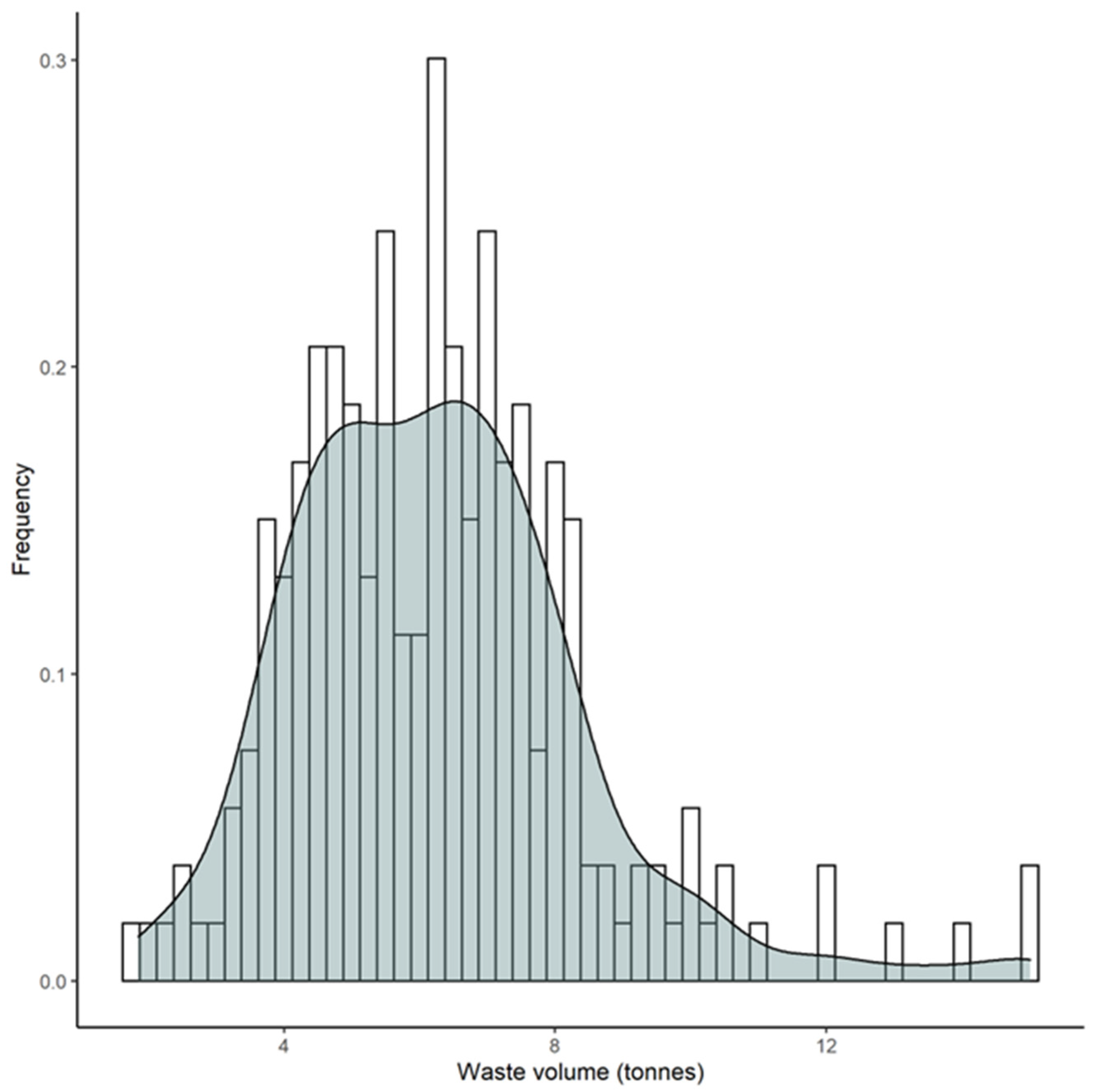
Figure 3.
Correlation analysis of variables.
Figure 3.
Correlation analysis of variables.
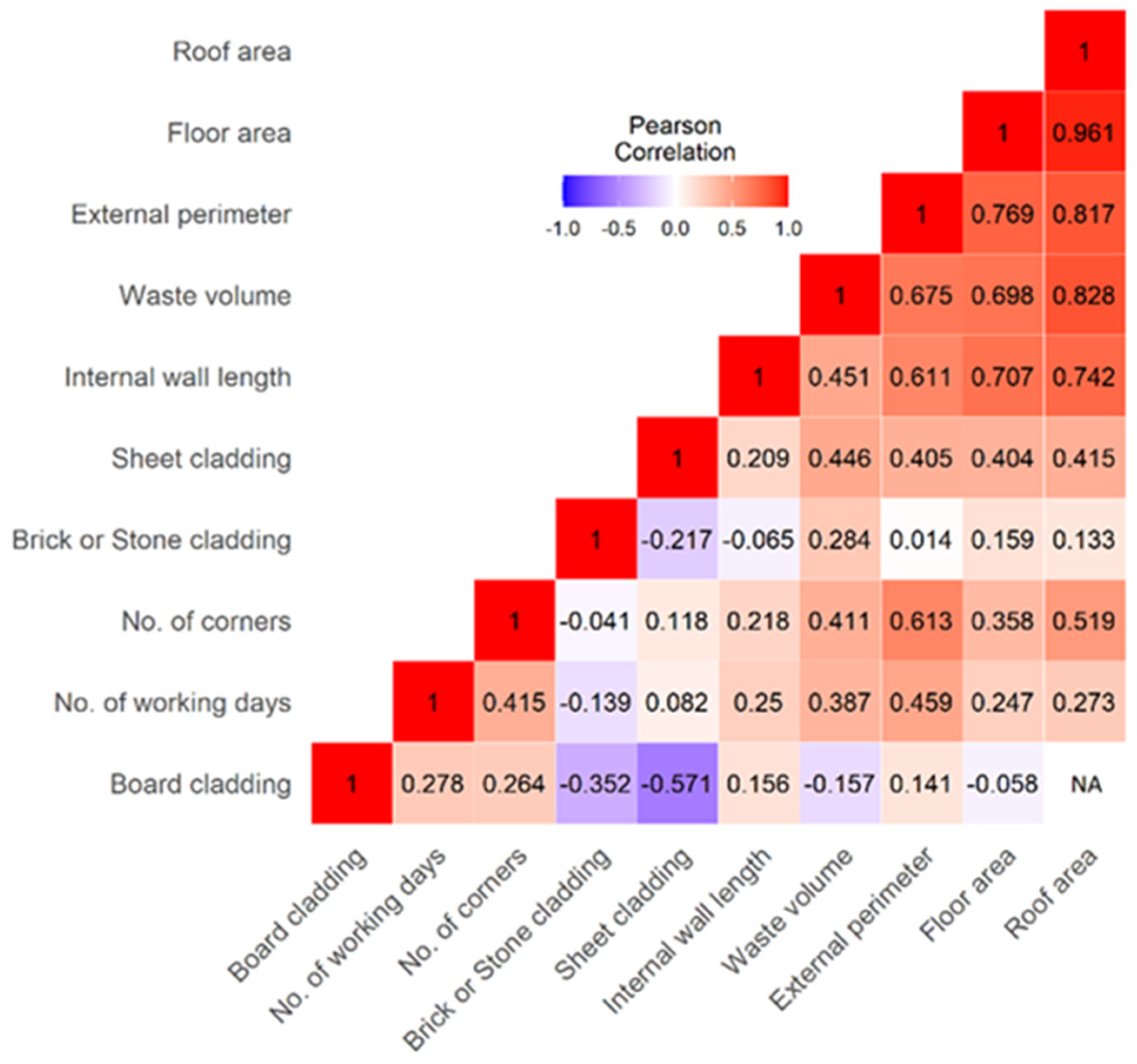
Table 1.
Summary of numerical variables.
Table 1.
Summary of numerical variables.
| Variables | n | Mean ± SD | Median | Minimum | Maximum | Skewness | Kurtosis |
|---|---|---|---|---|---|---|---|
| Response Variable | |||||||
| Waste volume (tonnes) | 213 | 6.28 ± 2.16 | 6.20 | 1.85 | 15.00 | 1.08 | 2.40 |
| Predictor Variables | |||||||
| Working days (days) | 213 | 139.02 ± 33.97 | 132.00 | 67.00 | 310.00 | 1.36 | 3.11 |
| Floor area (m2) | 213 | 192.38 ± 41.45 | 192.00 | 89.60 | 337.90 | 0.55 | 1.13 |
| External perimeter (m) | 213 | 72.95 ± 17.32 | 69.30 | 40.00 | 154.00 | 1.75 | 4.51 |
| Internal wall length (m) | 213 | 67.51 ± 19.88 | 63.00 | 13.00 | 165.00 | 1.19 | 3.49 |
| Corners (count) | 213 | 18.70 ± 6.50 | 17.00 | 9.00 | 46.00 | 1.43 | 2.30 |
| Board cladding (m2) | 213 | 50.92 ± 56.16 | 34.00 | 0.00 | 224.00 | 0.84 | −0.30 |
| Sheet cladding (m2) | 213 | 85.92 ± 75.38 | 77.00 | 0.00 | 384.00 | 0.70 | 0.35 |
| Brick or stone (m2) | 213 | 26.83 ± 55.81 | 0.00 | 0.00 | 240.00 | 2.00 | 2.83 |
| Roof area (m2) | 51 | 299.76 ± 51.26 | 291.00 | 211.00 | 460.00 | 0.94 | 1.51 |
Table 2.
Summary of categorical variables.
Table 2.
Summary of categorical variables.
| Category | Levels |
|---|---|
| House type | Single-family houses (n = 169) |
| Houses with a self-contained flat (n = 44) * | |
| Number of stories | 1 (n = 188) |
| 1.5 (n = 1) | |
| 2 (n = 24) | |
| Number of bathrooms | 1 (n = 6) |
| 1.5 (n = 1) | |
| 2 (n = 101) | |
| 2.5 (n = 39) | |
| 3 (n = 54) | |
| 3.5 (n = 7) | |
| 4 (n = 4) | |
| 5 (n = 1) | |
| Roof cladding type (for small builders only) | Pressed metal (n = 12) |
| Steel (n = 39) | |
| Builder type | National builder (n = 162) |
| Small builders (n = 51) |
Table 3.
Best-fitting generalised linear model (model 1) for residential buildings.
Table 3.
Best-fitting generalised linear model (model 1) for residential buildings.
| Estimate | Std. Error | t Value | p Value | |
|---|---|---|---|---|
| (Intercept) | 0.352 | 0.094 | 3.754 | 0.000 |
| Working days | 0.004 | 0.001 | 6.858 | 0.000 |
| Floor area | 0.003 | 0.000 | 6.868 | 0.000 |
| Number of corners | 0.008 | 0.003 | 2.905 | 0.004 |
| Builder type—small builders | 0.372 | 0.046 | 8.090 | 0.000 |
Table 4.
Selected list of models with more than 56% accuracy.
Table 4.
Selected list of models with more than 56% accuracy.
| Model Name | AIC | Accuracy of Prediction |
|---|---|---|
| Model 1: volume ~ working days + floor area + corners + type of builder | 516.28 | 56.00% |
| Model 2: volume ~ working days + floor area + internal wall length + external perimeter + board cladding + sheet cladding + brick or stone + stories + bathrooms + house type + corners + type of builder | 528.25 | 80% |
| Model 3: volume ~ stories + sheet cladding + PC1 + PC2 | 71.48 | 75.00% |
| Model 4: volume ~ working days + PC1 + PC2 + roof clad + sheet cladding + bathrooms + stories | 82.40 | 100.00% |
| Model 5: volume ~ working days + floor area + bathrooms + corners + type of builder | 72.00% | |
| Model 6: volume ~ working days + floor area + bathrooms + corners + type of builder + stories | 72.00% | |
| Model 7: volume ~ working days + floor area + bathrooms + corners + type of builder + house type | 72.00% | |
| Model 8: volume ~ working days + floor area + bathrooms + corners + type of builder + sheet cladding | 72.00% | |
| Model 9: volume ~ working days + floor area + bathrooms + corners + type of builder + sheet cladding + board cladding | 74.00% | |
| Model 10: volume ~ working days + floor area + bathrooms + corners + type of builder + sheet cladding + board cladding | 78.00% |
Table 5.
Principal component analysis of built area for subset2.
Table 5.
Principal component analysis of built area for subset2.
| PC1 | PC2 | |
|---|---|---|
| Eigenvalue | 3.57 | 0.30 |
| Variance explained | 89.93 | 7.41 |
| Loading scores: | ||
| Floor area | −0.52 | −0.33 |
| External perimeter | −0.51 | 0.29 |
| Internal wall length | −0.48 | 0.67 |
| Roof area | −0.49 | −0.60 |
Table 6.
Generalised linear model (model 2) without roof parameters.
Table 6.
Generalised linear model (model 2) without roof parameters.
| Estimate | Std. Error | t Value | p Value | |
|---|---|---|---|---|
| (Intercept) | 0.609 | 0.165 | 3.682 | 0.000 |
| Working days | 0.003 | 0.001 | 4.103 | 0.000 |
| Floor area | 0.002 | 0.001 | 2.741 | 0.007 |
| Internal wall length | −0.001 | 0.001 | −0.463 | 0.644 |
| External perimeter | 0.002 | 0.003 | 0.755 | 0.451 |
| Board cladding area | 0.000 | 0.001 | 0.334 | 0.739 |
| Sheet cladding area | 0.000 | 0.001 | 0.710 | 0.479 |
| Brick or stone cladding area | 0.001 | 0.001 | 1.313 | 0.191 |
| Number of stories—2 | 0.094 | 0.092 | 1.017 | 0.311 |
| Number of bathrooms | ||||
| 2 | −0.183 | 0.127 | −1.442 | 0.151 |
| 2.5 | −0.286 | 0.143 | −1.994 | 0.048 |
| 3 | −0.162 | 0.142 | −1.141 | 0.256 |
| 3.5 | −0.236 | 0.170 | −1.388 | 0.167 |
| 4 | −0.202 | 0.230 | −0.875 | 0.383 |
| House type | 0.073 | 0.065 | 1.135 | 0.258 |
| Number of corners | 0.008 | 0.004 | 2.212 | 0.029 |
| Builder type—Small builders | 0.367 | 0.076 | 4.861 | 0.000 |
Table 7.
Best-fitting generalised linear model (model 3) for waste volume with roof parameters.
Table 7.
Best-fitting generalised linear model (model 3) for waste volume with roof parameters.
| Estimate | Std. Error | t Value | p Value | |
|---|---|---|---|---|
| (Intercept) | 2.00 | 0.02 | 95.60 | 0.00 |
| Stories—2 | 0.26 | 0.08 | 3.35 | 0.00 |
| Sheet cladding area | 0.00 | 0.00 | 1.79 | 0.08 |
| PC1 | −0.09 | 0.01 | −10.42 | 0.00 |
| PC2 | −0.05 | 0.02 | −2.15 | 0.04 |
Table 8.
Generalised linear model (model 4) with roof parameters.
Table 8.
Generalised linear model (model 4) with roof parameters.
| Estimate | Std. Error | t Value | p Value | |
|---|---|---|---|---|
| (Intercept) | 2.040 | 0.044 | 45.989 | 0.000 |
| Working days | 0.000 | 0.000 | −0.237 | 0.814 |
| PC1 | −0.095 | 0.017 | −5.460 | 0.000 |
| PC2 | −0.060 | 0.039 | −1.520 | 0.138 |
| Roof cladding type | −0.003 | 0.026 | −0.123 | 0.903 |
| Sheet cladding area | 0.000 | 0.000 | 1.672 | 0.104 |
| Number of bathrooms | ||||
| 2.5 | −0.044 | 0.025 | −1.800 | 0.081 |
| 3 | −0.043 | 0.157 | −0.274 | 0.786 |
| 3.5 | 0.050 | 0.098 | 0.509 | 0.614 |
| Number of stories—2 | 0.217 | 0.154 | 1.415 | 0.166 |
Table 9.
Predicted values from ensemble models of the prediction tool.
Table 9.
Predicted values from ensemble models of the prediction tool.
| Model 2 | Model 3 | Average Predictions | Actual Waste Volume | ||||||
|---|---|---|---|---|---|---|---|---|---|
| Prediction | Lower Limit | Upper Limit | Prediction | Lower Limit | Upper Limit | Prediction | Lower Limit | Upper Limit | |
| 6.96 | 5.75 | 8.42 | 7.10 | 6.44 | 7.83 | 7.03 | 6.10 | 8.13 | 7.00 |
| 6.81 | 5.82 | 7.96 | 7.68 | 7.14 | 8.26 | 7.24 | 6.48 | 8.11 | 7.25 |
| 6.76 | 5.81 | 7.88 | 7.38 | 6.91 | 7.89 | 7.07 | 6.36 | 7.88 | 7.00 |
| 7.17 | 6.16 | 8.35 | 7.55 | 7.02 | 8.11 | 7.36 | 6.59 | 8.23 | 7.25 |
| 6.08 | 5.23 | 7.06 | 6.67 | 6.06 | 7.35 | 6.38 | 5.65 | 7.21 | 6.50 |
| 6.88 | 5.69 | 8.32 | 7.06 | 6.42 | 7.76 | 6.97 | 6.06 | 8.04 | 7.50 |
| 8.11 | 6.93 | 9.49 | 8.09 | 7.47 | 8.76 | 8.10 | 7.20 | 9.13 | 8.00 |
| 7.68 | 6.48 | 9.10 | 6.94 | 6.36 | 7.57 | 7.31 | 6.42 | 8.33 | 7.50 |
|
Disclaimer/Publisher’s Note: The statements, opinions and data contained in all publications are solely those of the individual author(s) and contributor(s) and not of MDPI and/or the editor(s). MDPI and/or the editor(s) disclaim responsibility for any injury to people or property resulting from any ideas, methods, instructions or products referred to in the content. |
[ad_2]