Three-Dimensional Quantification and Visualization of Leaf Chlorophyll Content in Poplar Saplings under Drought Using SFM-MVS

By inergency On Jan 6, 2024

[ad_1]

Figure 1.
Schematic diagram of multi-view image acquisition. Illustration: (a) Image acquisition system diagram; (b) On-site work demonstration.

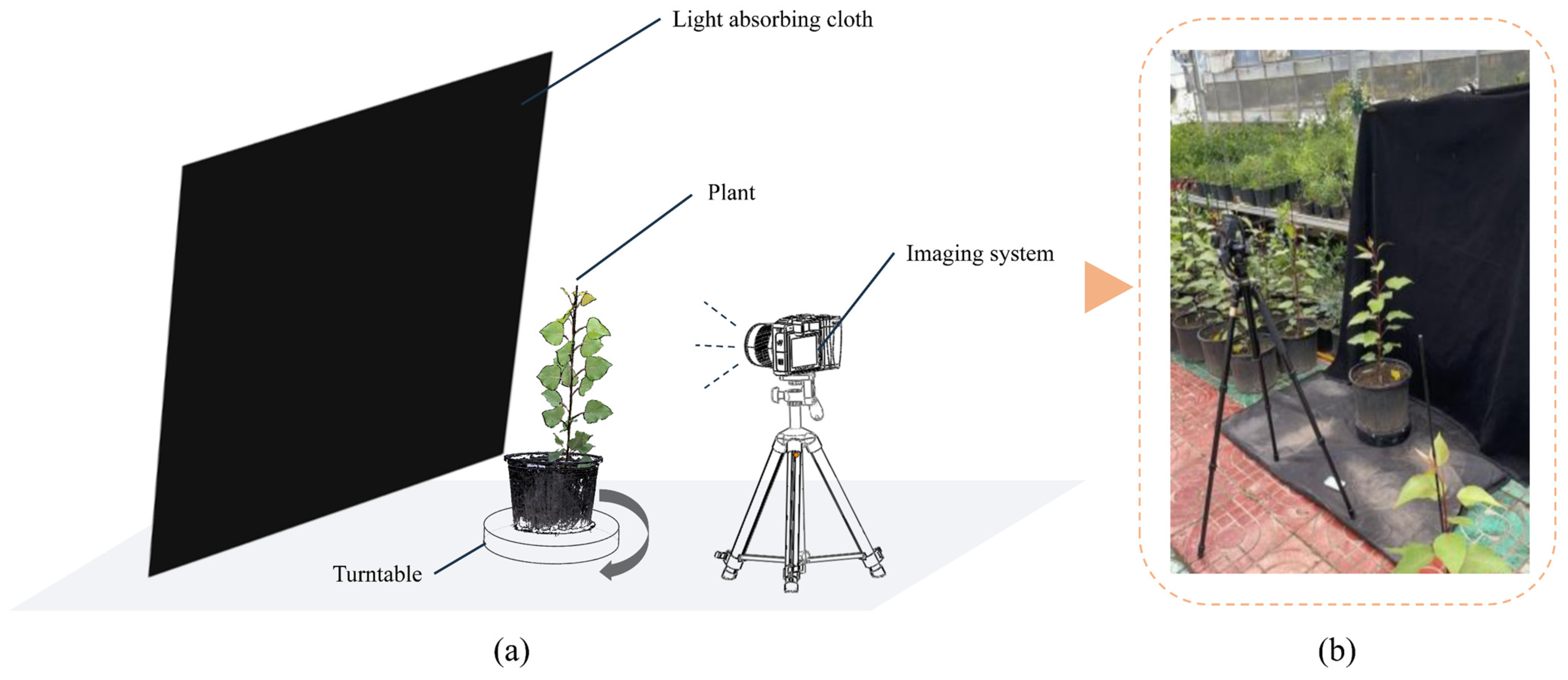
Figure 2.
Image pre-processing before 3D reconstruction. Illustration: (a,b) represent image correction and denoising, respectively. Where, (1) raw image, (2) image white balance, color and distortion correction, (3) corrected image, (4) excess green calculation, (5) threshold segmentation, (6) image opening operation, (7) processed image.

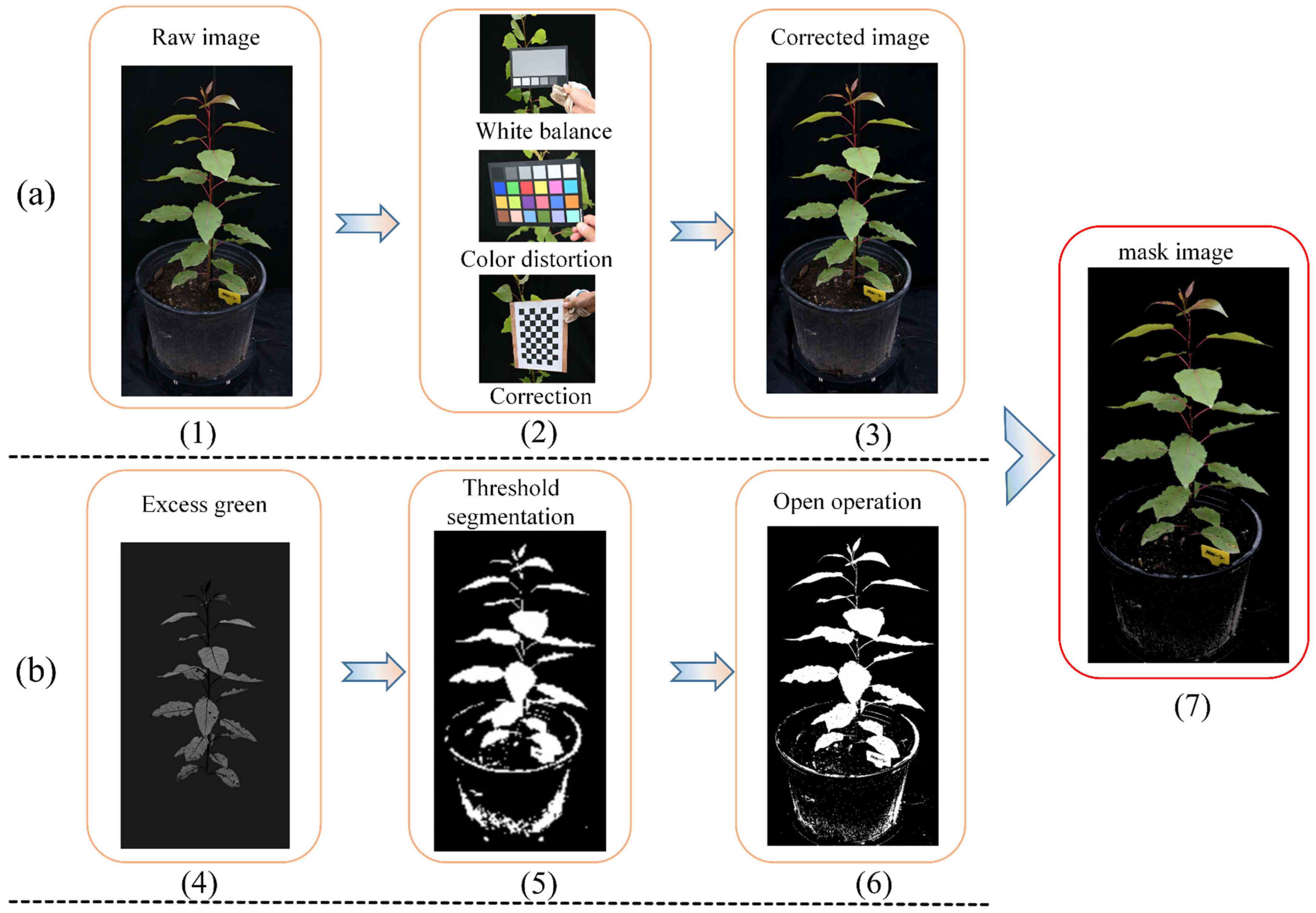
Figure 3.
Plant point cloud reconstruction based on SFM-MVS. Illustration: (a) Image sequence after noise reduction; (b) Sparse point cloud reconstruction; (c) Dense point cloud reconstruction.

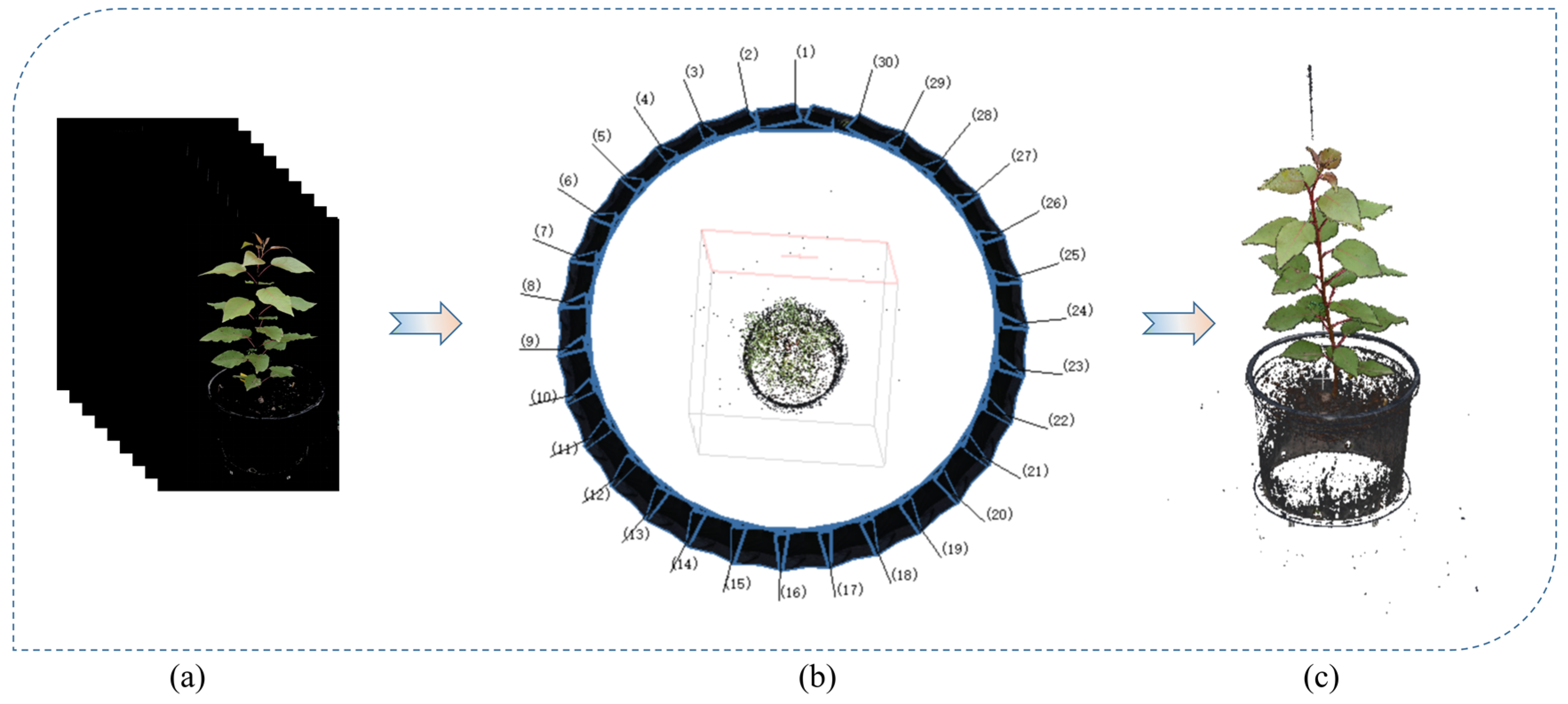
Figure 4.
Point cloud noise reduction based on different filter functions. Illustration: (a) Spatial filtered point cloud; (b) Point cloud after color filtering; (c) Point cloud after radius filtering.

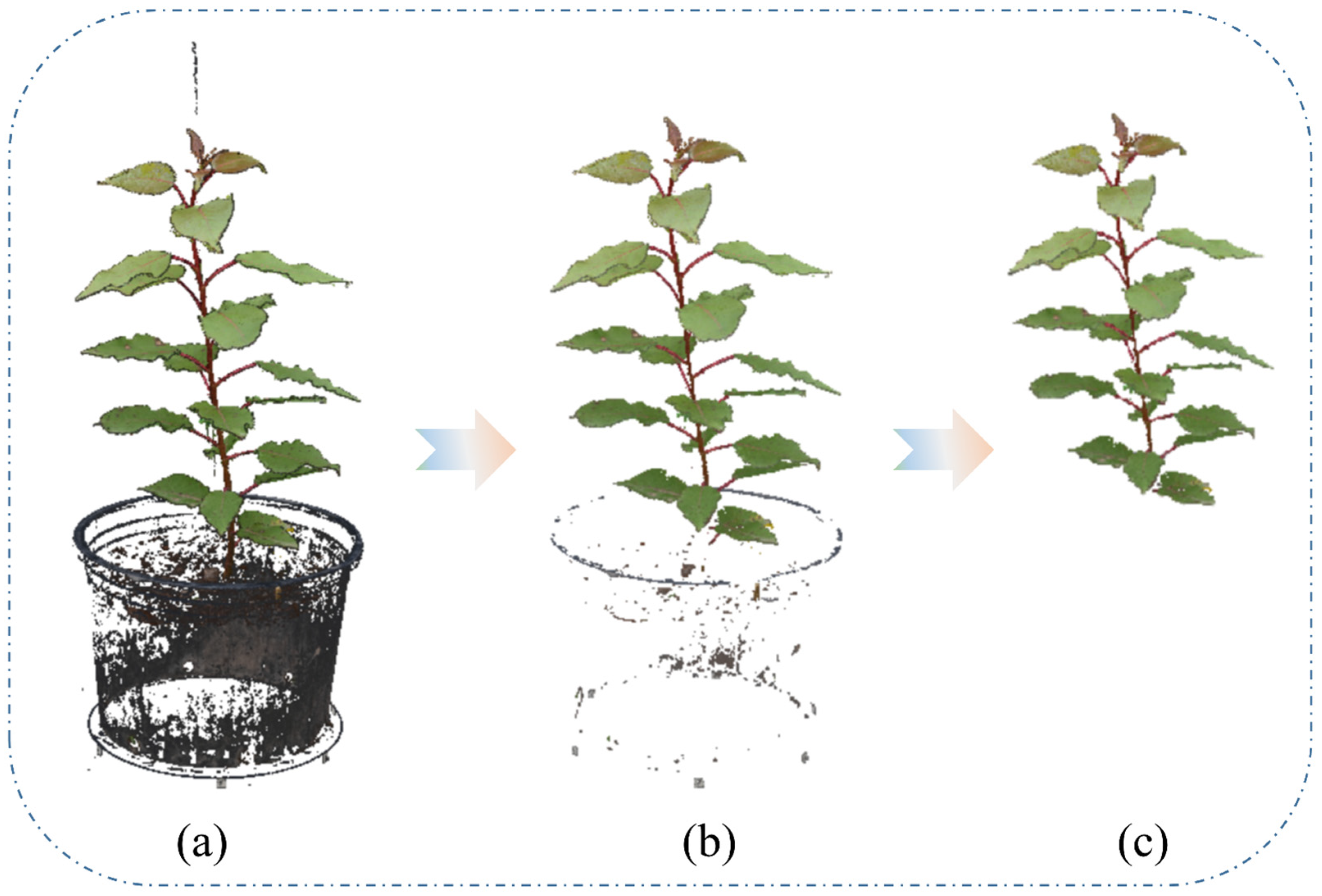
Figure 5.
Point cloud shape and size calibration.

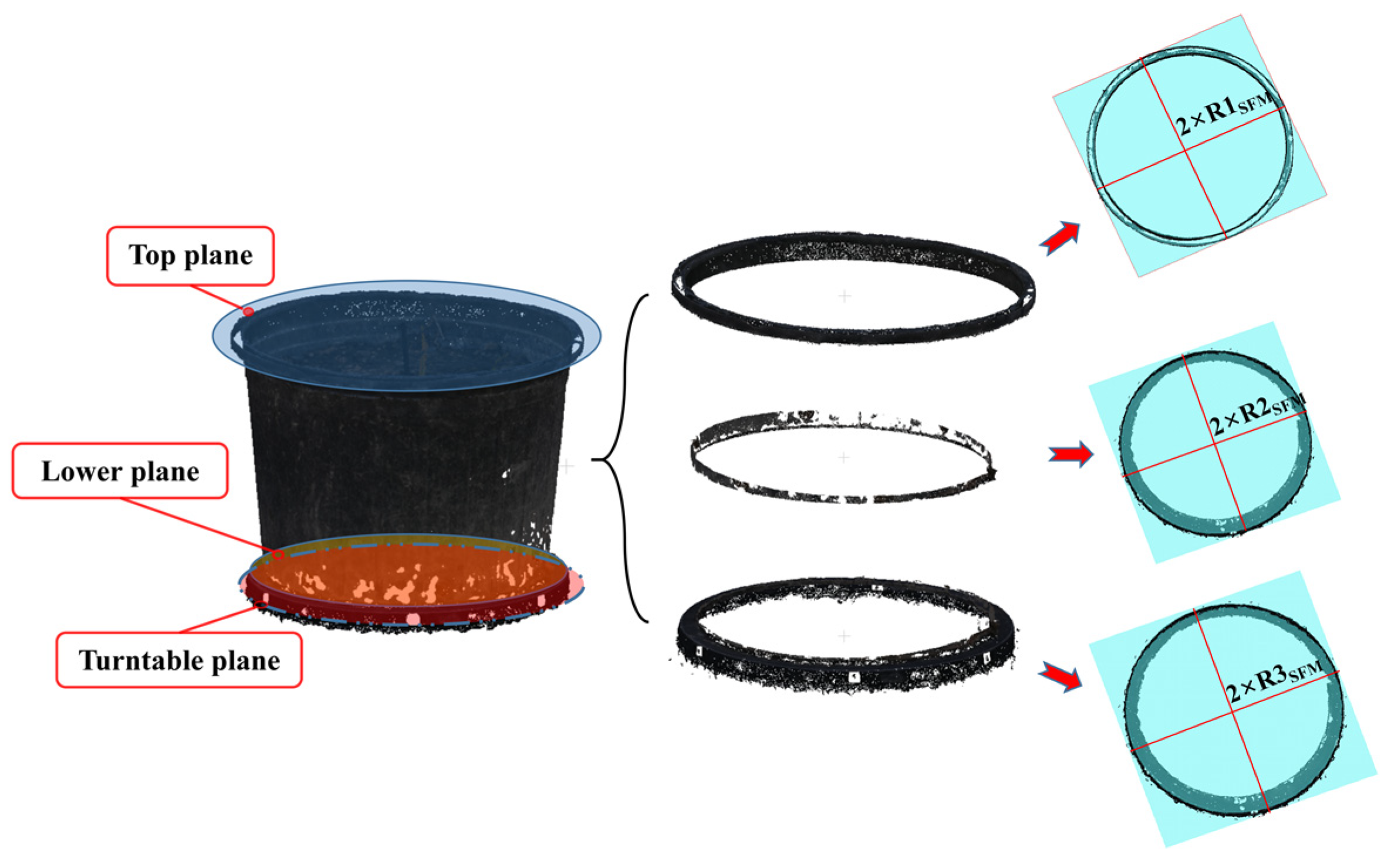
Figure 6.
Processing flow of 3D distribution of poplar chlorophyll. Illustration: (a) Raw image; (b) Blade stratification; (c) Color feature extraction; (d) Variable selection; (e) model regression; (f) Visualization.

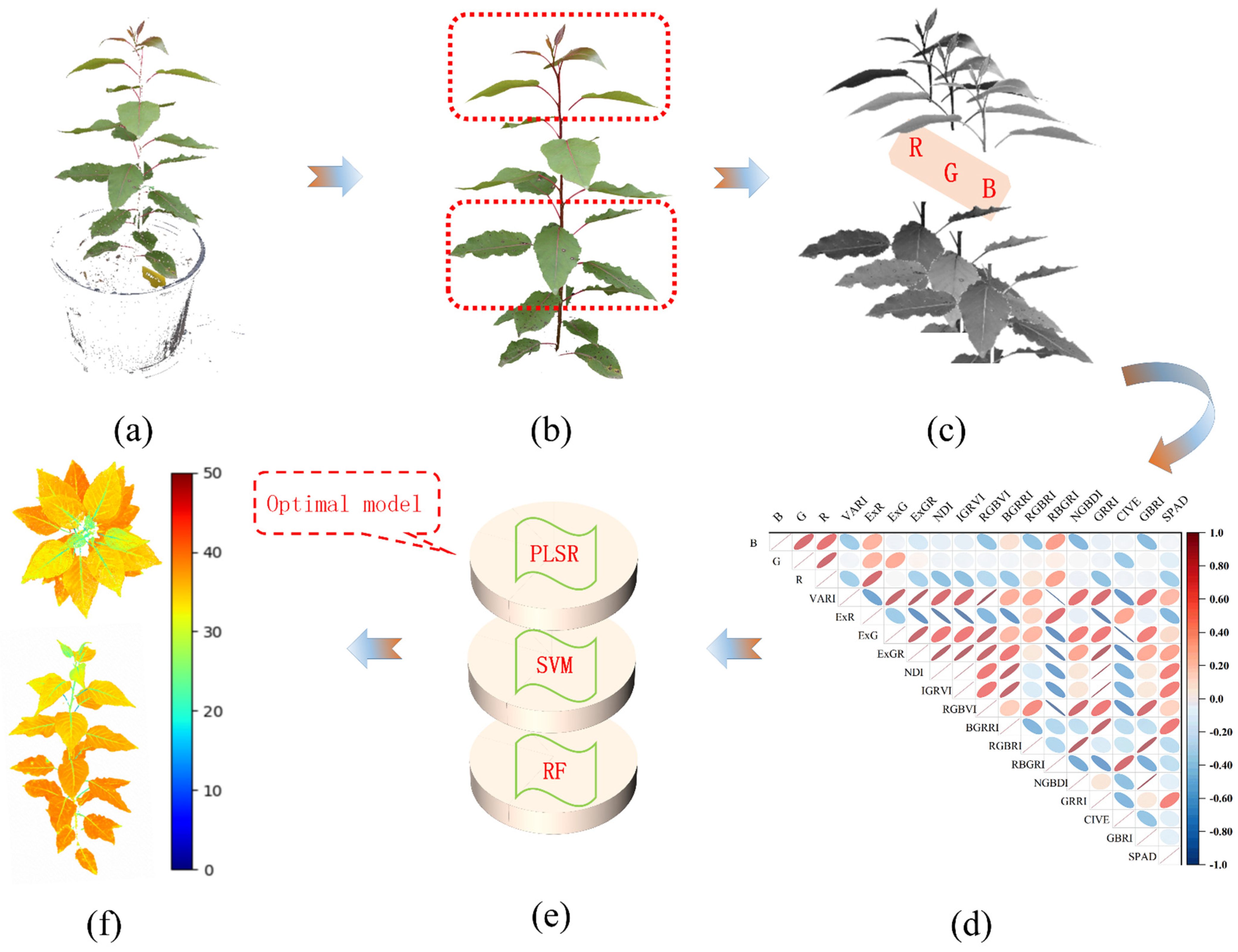
Figure 7.
Calculation of color information of poplar stratified leaves. Illustration: P is the pixel value of R, G and B of a certain blade, n is the number of times the box of interest is selected; α(β) is the average pixel value of R, G, and B of the top (lower) leaves of a single poplar tree, η_Top(η_Lower) is the average pixel value of R, G, and B in the top (lower) layer of a single poplar tree.

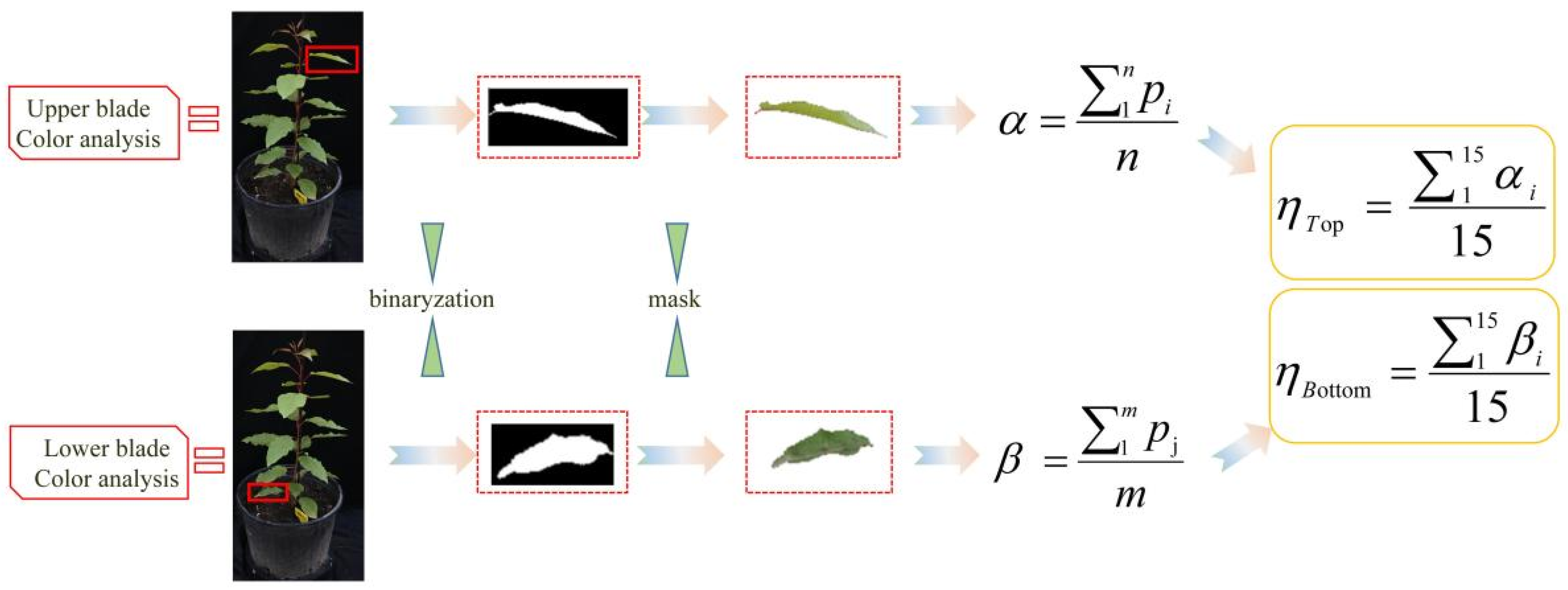
Figure 8.
Regression results of each model. Illustration: (a) RF; (b) SVM; (c) PLSR.

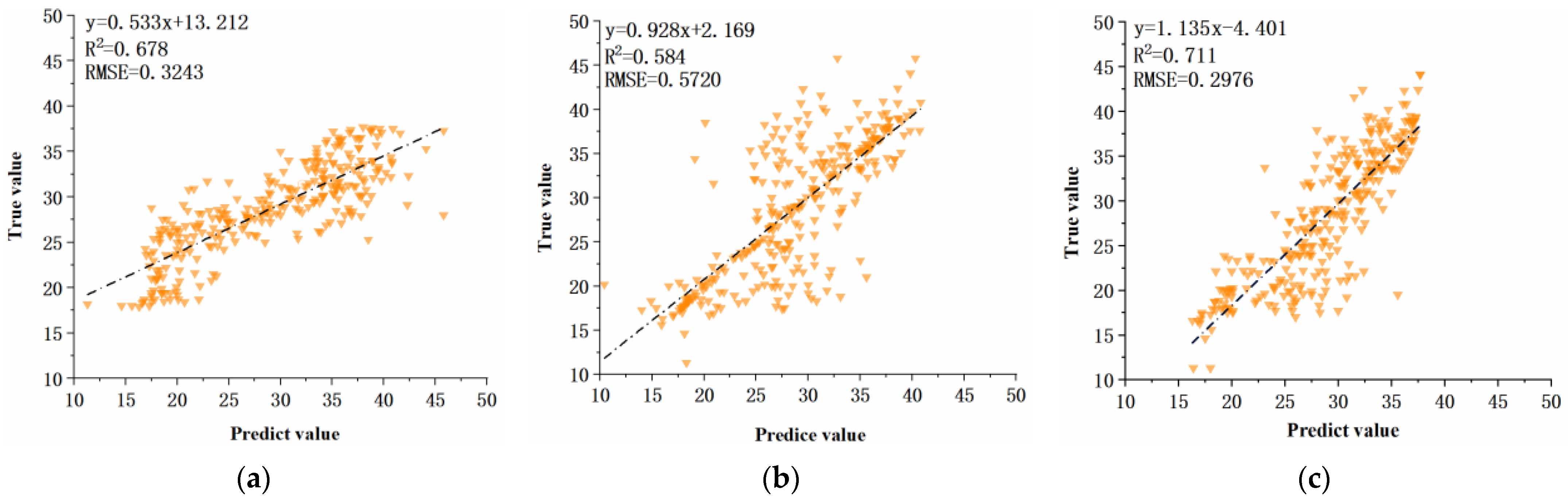
Figure 9.
Chlorophyll three-dimensional visualization at each stage of the test. (a) 3D visualization of poplar chlorophyll at different growth stages (Illustration: Pictures (1), (2), (3), and (4), respectively, correspond to the three-dimensional chlorophyll visualization model of the same plant from week 1 to week 4). (b) 3D visualization of 110poplar chlorophyll under different water treatments (Illustration: Pictures (5), (6), and (7), respectively, correspond to the three-dimensional chlorophyll visualization model of the same genotype (110) under different drought treatment levels). (c) Three-dimensional visualization of chlorophyll under different gene regulation (Illustration: Pictures (8), (9), (10), and (11), respectively, correspond to the three-dimensional chlorophyll visualization points of the four poplar varieties 3804, 110, SY-1, and 895 from before drought treatment (upper dotted line box) to after drought treatment (lower dotted line box) cloud model).

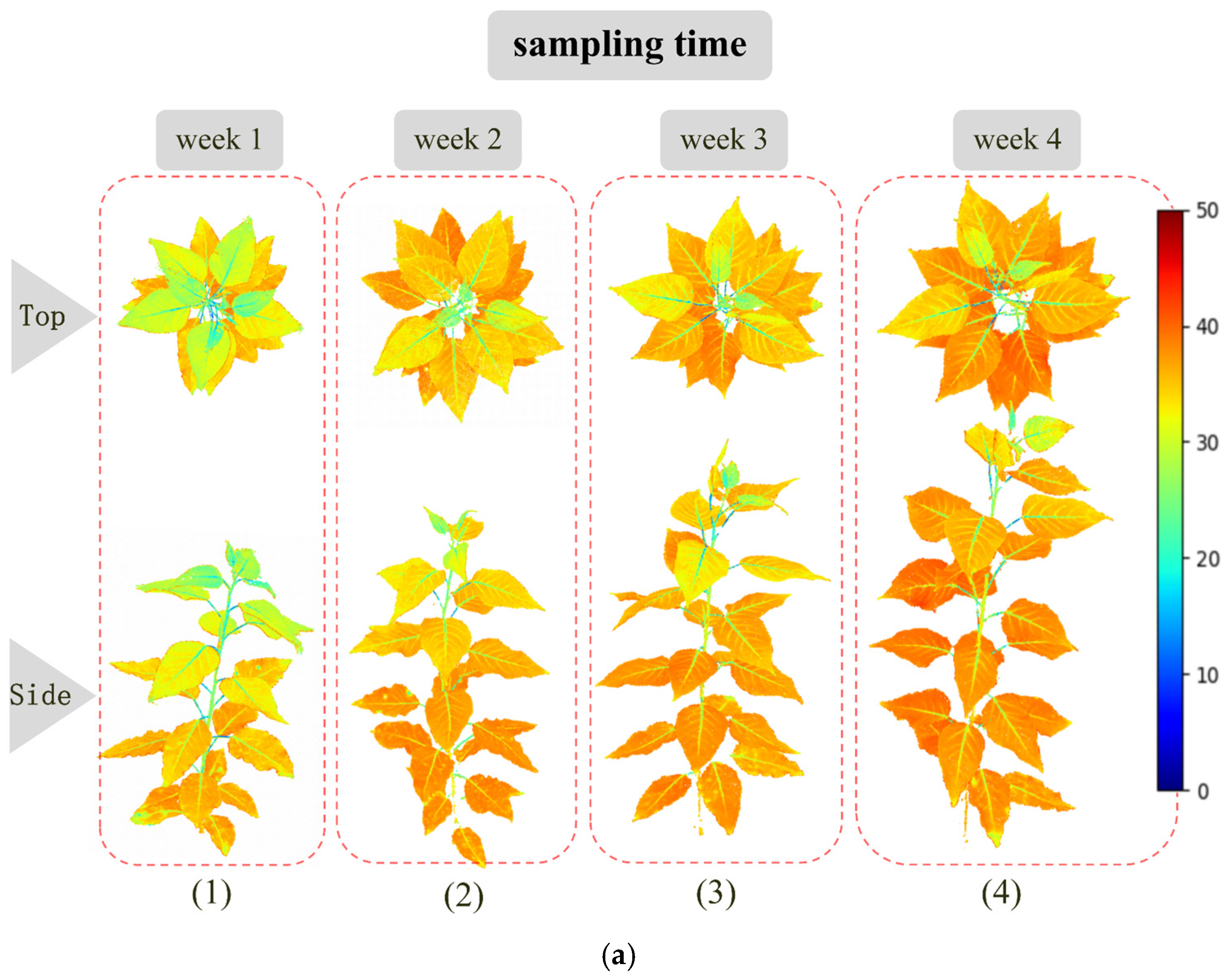
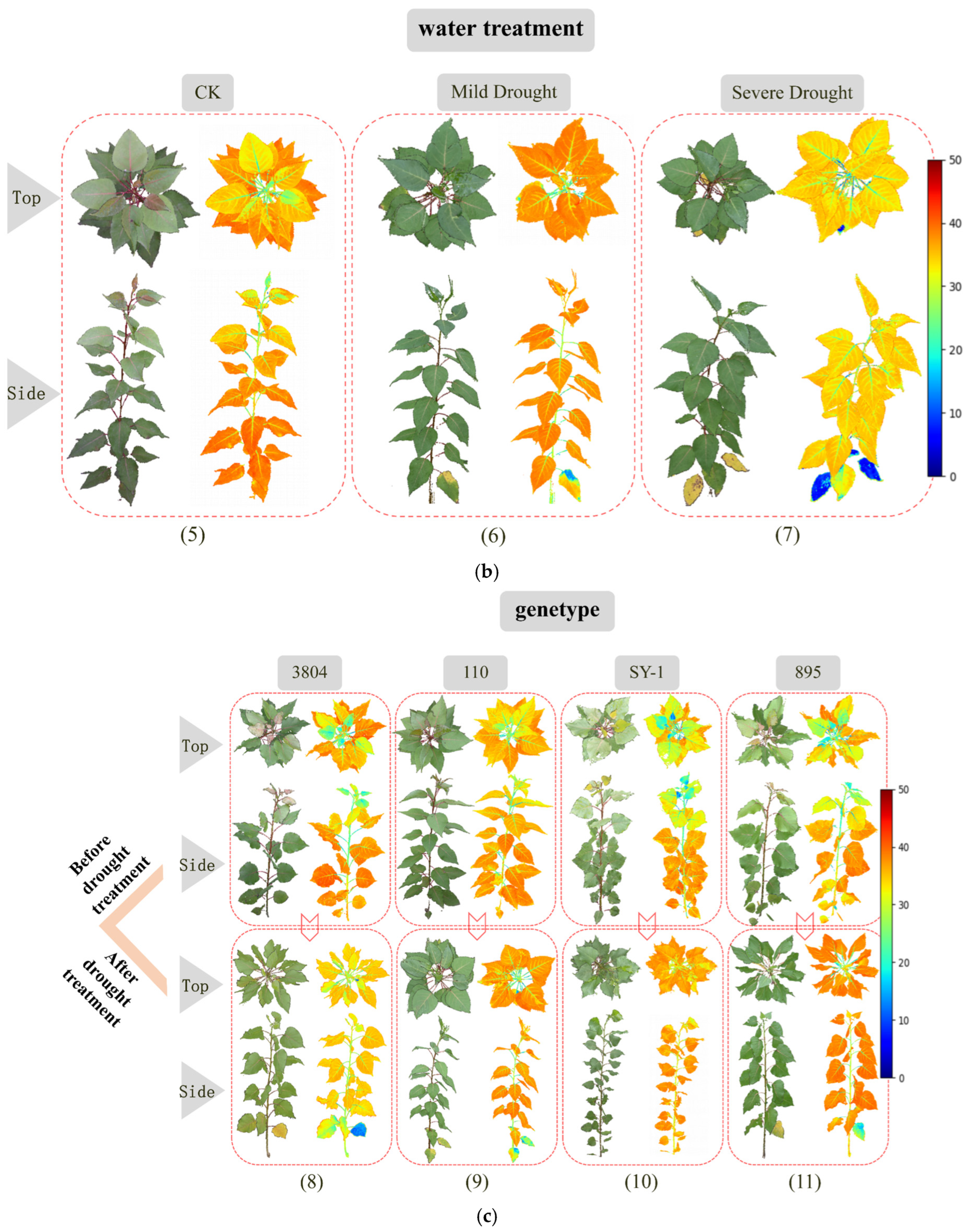
Figure 10.
Chlorophyll content response at each stage of the test. Illustration: CK, mild drought, and severe drought in the figure represent the three levels of drought culture, respectively; top and lower represents upper leaves and lower leaves, and the time when drought begins is the 28th to 43rd day after the start of the experiment.

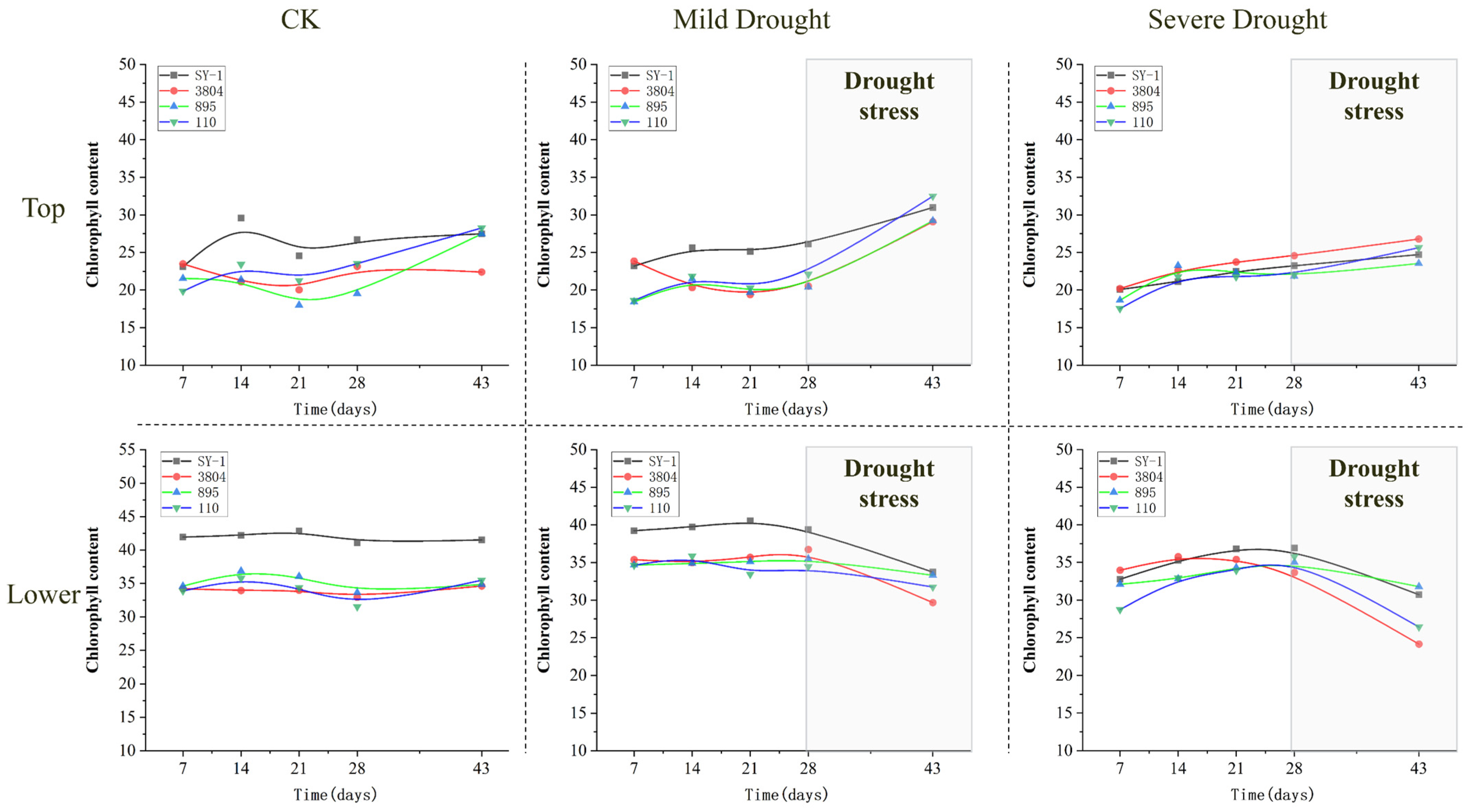
Table 1.
General profile of the experiment.

	Before Drought Treatment	After Drought Treatment
Image acquisition times	4	1
Experiment sample size	96	Control check	Mild drought	Severe drought
Experiment sample size	96	32	32	32
Experiment interval date (days)	7	15

Table 2.
Camera models and parameters for acquiring multi-view images.

Specific Parameters (Symbol)	Camera Model Nikon Z5
Specific Parameters (Symbol)	Numerical Value	Unit
Shutter speed (S)	1/320	Seconds (s)
Aperture (A)	10	Dimensionless
Speed (ISO)	100	Dimensionless
Imaging focal length (f)	35	Millimeter (mm)
Image storage format (F)	JPG	Dimensionless
Picture size (P)	4016 × 6016	Pixels per inch (PPI)
Total rotation Angle (θ)	400	Degree (°)

Table 3.
Point cloud filter noise reduction function parameter setting.

Function Type	Parameter Setting
Spatial filtering	X (m)	Y (m)	Z (m)
Spatial filtering	0.65	0.65	1.5
Color filtering	R	G	B
Color filtering	60	60	60
Radius filtering	r (mm)		n (a)
Radius filtering	0.5		20

Table 4.
Vegetation indices developed from RGB images.

Color Index Type	Color Index Name	Abbreviation	Formula
Normalized type color index	(visible-band difference vegetation index)	VDVI	$(2 G - R - B) / (2 G + R + B)$
	(normalized green-blue difference index)	NGBDI	$(G - B) / (G + B)$
	(visible atmospheric impedance vegetation index)	VARI	$(G - R) / (G + R - B)$
	(normalized difference index)	NDI	$(G - R) / (G + R)$
	(improved green-red vegetation index)	IGRVI	$(G - R^{2}) / (G + R^{2})$
	(red-green-blue vegetation index)	RGBVI	$(G^{2} - B R) / (G^{2} + B R)$
Ratio type color index	(green-red ration index)	GRRI	$G / R$
	(blue-green red ration index)	BGRRI	$(G + B) / R$
	(red-green blue ration index)	RGBRI	$(G + R) / B$
	(red-blue green ration index)	RBGRI	$(R + B) / G$
Composite color index	(excess green index)	ExG	$2 G - R - B$
	(excess red index)	ExR	$1.4 R - G$
	(green-red difference vegetation index)	ExGR	$E x G - E x R$
	(color index of vegetation)	CIVE	$0.411 R - 0.881 + 0.385 + 18.7578$

[ad_2]