Effects of Understory Vegetation Conversion on Soil Greenhouse Gas Emissions and Soil C and N Pools in Chinese Hickory Plantation Forests
[ad_1]
Figure 1.
(a,b) Schematic of the location of the test sample plots. (c) Distribution map of the test sample plots; (d) size and spacing distance of each sample plot; (e) Chinese hickory test subjects in the test sample plots; (f) field soil GHG collection tool.
Figure 1.
(a,b) Schematic of the location of the test sample plots. (c) Distribution map of the test sample plots; (d) size and spacing distance of each sample plot; (e) Chinese hickory test subjects in the test sample plots; (f) field soil GHG collection tool.
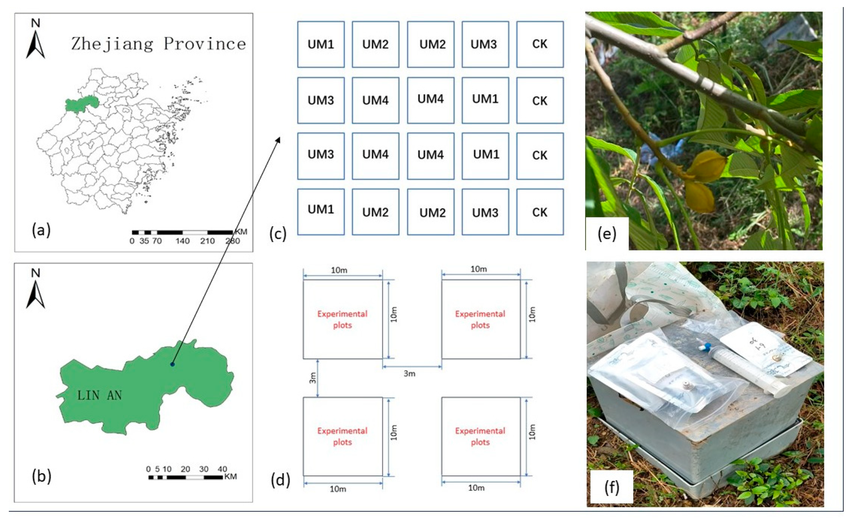
Figure 2.
Effects of different understory vegetation modifications on (a) CO2, (b) N2O, and (c) CH4 uptake from Chinese hickory plantation soils. Standard deviations are indicated by error lines.
Figure 2.
Effects of different understory vegetation modifications on (a) CO2, (b) N2O, and (c) CH4 uptake from Chinese hickory plantation soils. Standard deviations are indicated by error lines.
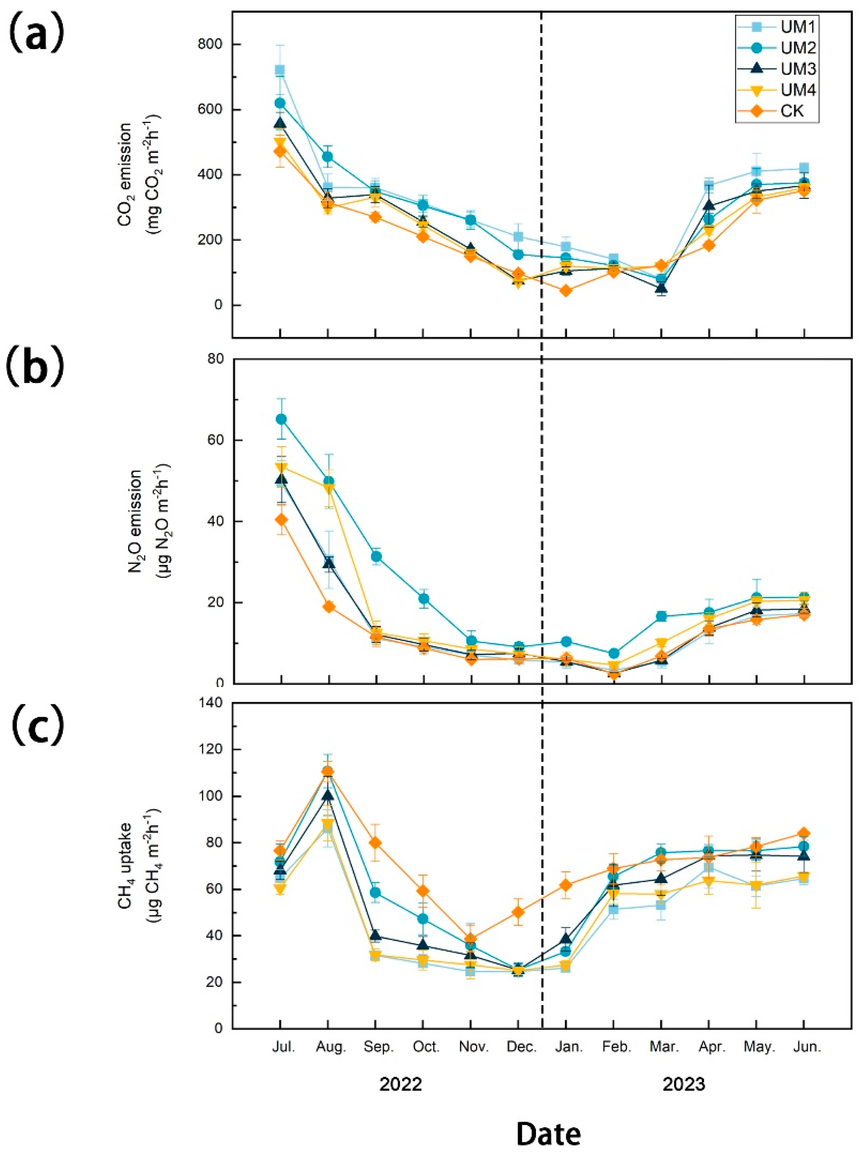
Figure 3.
Effects of different understory vegetation modifications on annual cumulative (a) CO2 emissions, (b) N2O emissions, (c) CH4 uptake, and (d) total soil GHG emissions from Chinese hickory plantation soils. Standard deviations are indicated by error lines. The letters a, b, c, and d are the distinctive symbols of annual emissions or annual absorption.
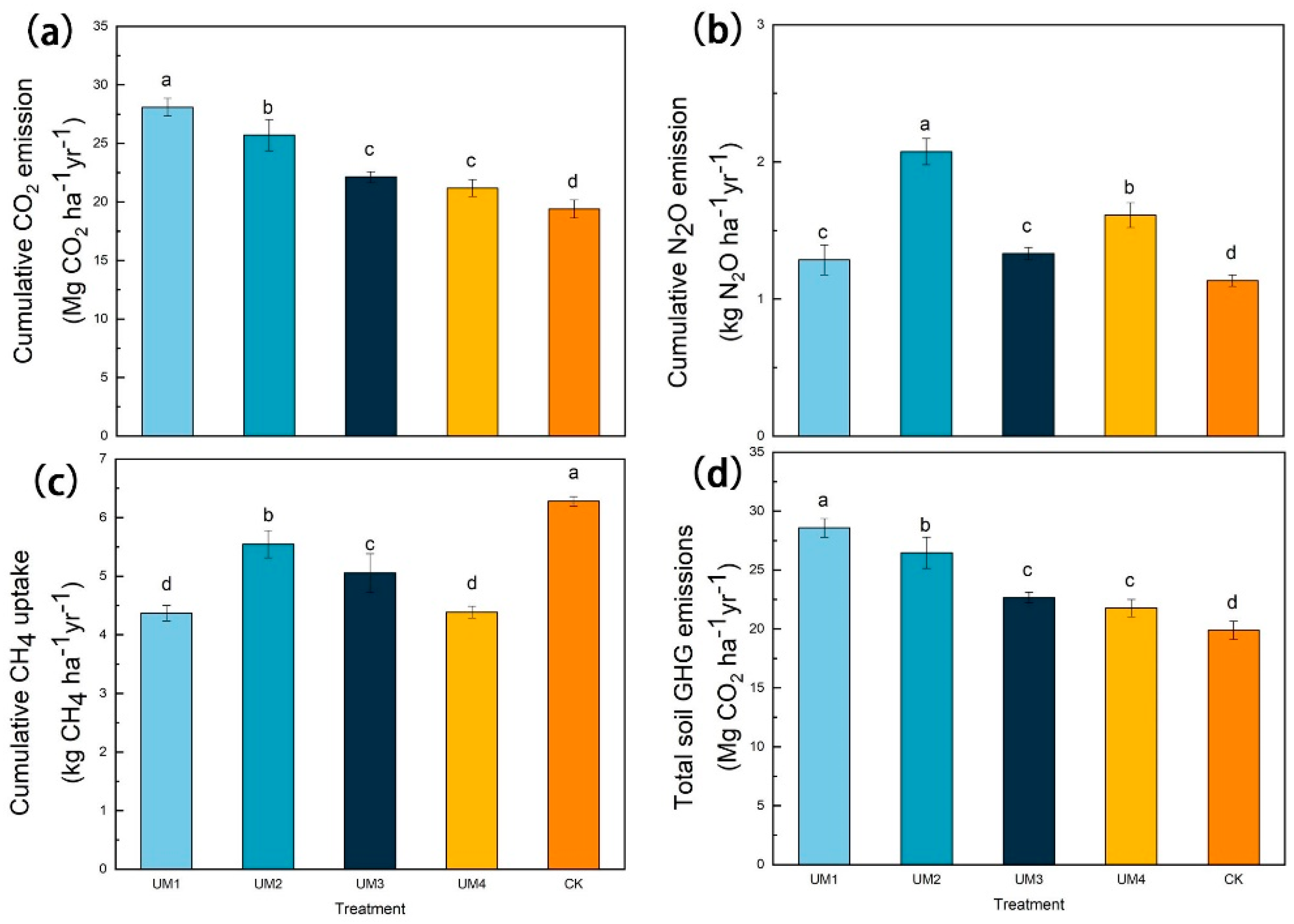
Figure 4.
Effects of different understory management on (a) 5 cm temperature, (b) soil moisture, and (c) pH of Chinese hickory plantation soils. Standard deviations are indicated by error lines.
Figure 4.
Effects of different understory management on (a) 5 cm temperature, (b) soil moisture, and (c) pH of Chinese hickory plantation soils. Standard deviations are indicated by error lines.
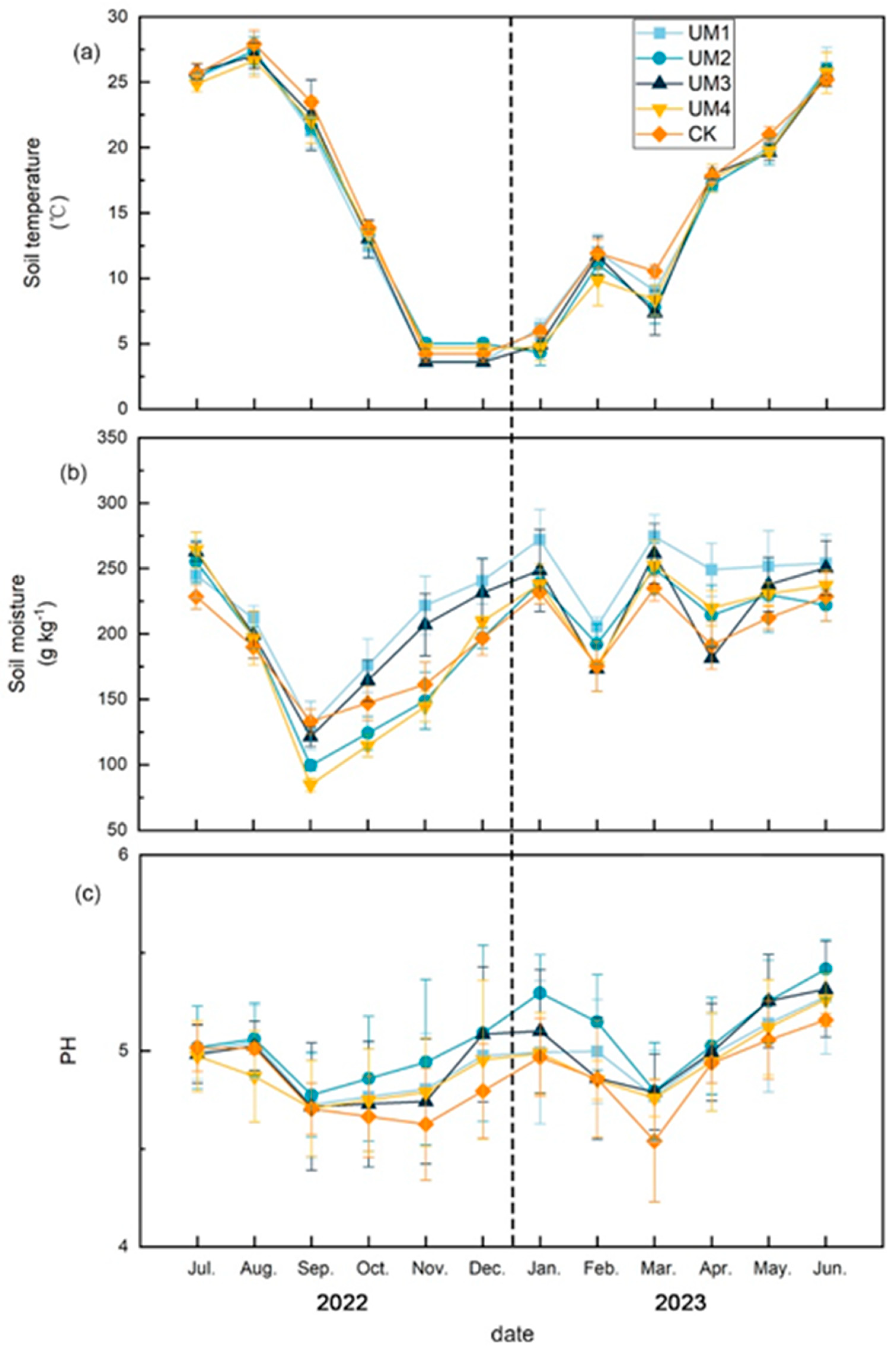
Figure 5.
Effects of different understory management on (a) WSOC and (b) MBC content of Chinese hickory plantation soils. Standard deviations are indicated by error lines.
Figure 5.
Effects of different understory management on (a) WSOC and (b) MBC content of Chinese hickory plantation soils. Standard deviations are indicated by error lines.
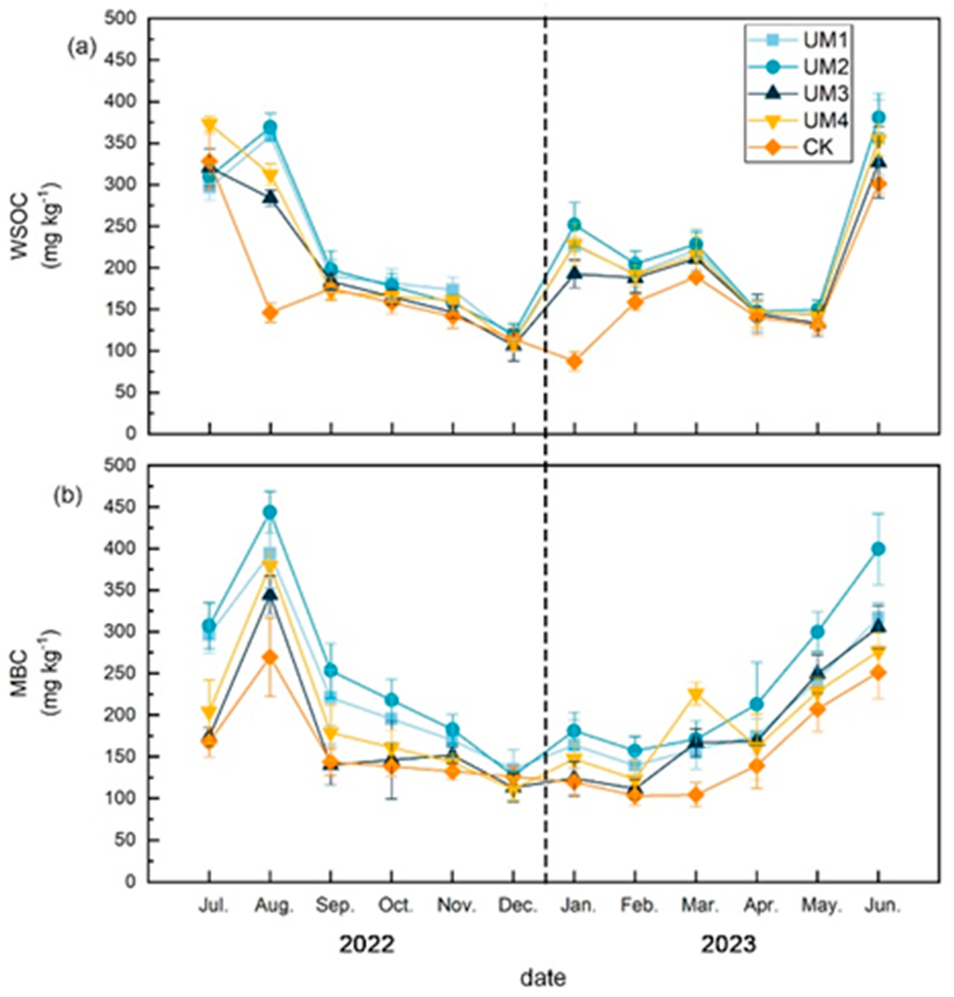
Figure 6.
Effects of different understory management conditions on (a) NO3−–N, (b) NH4+–N, (c) WSON, and (d) MBN contents of Chinese hickory plantation soils. Standard deviations are indicated by error lines.
Figure 6.
Effects of different understory management conditions on (a) NO3−–N, (b) NH4+–N, (c) WSON, and (d) MBN contents of Chinese hickory plantation soils. Standard deviations are indicated by error lines.
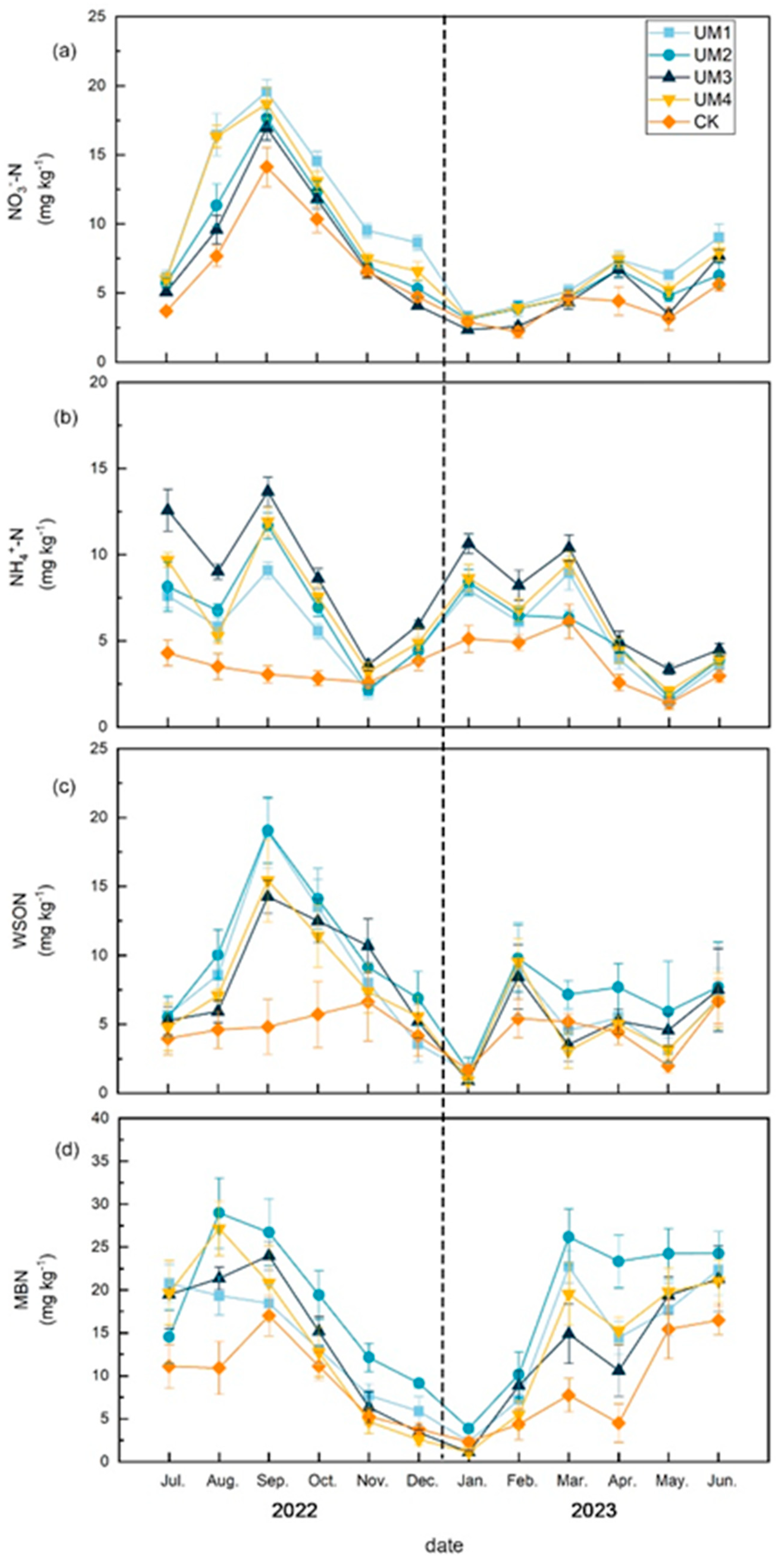
Figure 7.
Structural equation modelling of soil WSOC, MBC, NO3−–N, NH4+–N, WSON, and MBN concentrations affecting (a) CO2, (b) NO2, and (c) CH4 fluxes after forest understory vegetation conversion. Numbers next to arrows indicate correlation coefficients and significance. R2 indicates the rate of model explanation, GFI is the goodness-of-fit index, NFI is the normative fit index, and CFI is the comparative fit index.
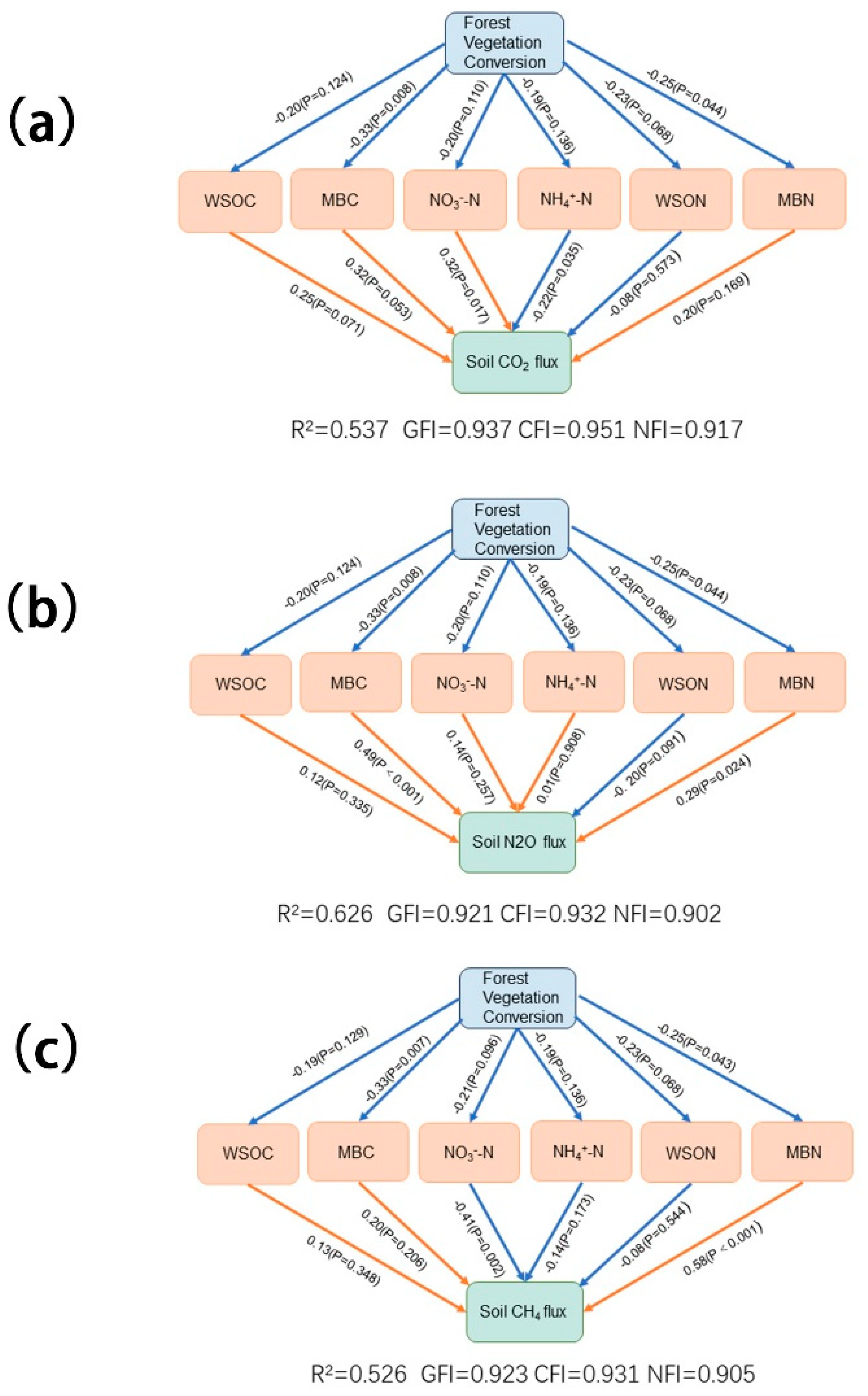
Table 1.
Weather and environmental conditions in Lin’an, Hangzhou, Zhejiang, China, from July 2022 to June 2023: average monthly temperature (°C), monthly precipitation (mm).
Table 1.
Weather and environmental conditions in Lin’an, Hangzhou, Zhejiang, China, from July 2022 to June 2023: average monthly temperature (°C), monthly precipitation (mm).
| Weather Environment | 2022 | 2023 | ||||||||||
|---|---|---|---|---|---|---|---|---|---|---|---|---|
| Jul. | Aug. | Spe. | Oct. | Nov. | Dec | Jan. | Feb. | Mar. | Apr. | May. | Jun. | |
| Average monthly temperature (°C) | 30.5 | 31 | 24 | 17.5 | 15 | −4.5 | −5.5 | 7 | 12.5 | 17 | 21.5 | 25.5 |
| Precipitation (mm) | 68.2 | 20 | 25.8 | 47.4 | 27.3 | 42.9 | 55.5 | 63.3 | 50.4 | 137.5 | 121.1 | 204.6 |
Table 2.
Stepwise regression analysis model between CO2 flux (mg m−2 h−1) and soil temperature (T, °C), soil moisture (M, g kg−1), water-soluble organic C (WSOC, mg kg−1), microbial biomass C (MBC, mg kg−1), NO3−–N, and NH4+–N under the UM1, UM2, UM3, UM4, and CK treatments. N, water-soluble organic N (WSON, mg kg−1), and microbial biomass N (MBN, mg kg−1) were modelled in a stepwise regression analysis. Coefficients in the model are standardized. R2 indicates the rate of model explanation.
| GHG | Treatment | Model | df | R2 | p |
|---|---|---|---|---|---|
| CO2 | UM1 | Y = 0.745T | 48 | 0.545 | ** |
| Y = 0.826T − 0.222WSON | 48 | 0.579 | ** | ||
| Y = 1.018T − 0.278WSON − 273WSOC | 48 | 0.615 | ** | ||
| Y = 1.251T − 0.392WSON − 426WSOC + 0.282NH4+–N | 48 | 0.662 | ** | ||
| UM2 | Y = 0.857T | 48 | 0.729 | ** | |
| Y = 1.044T − 0.303MBN | 48 | 0.783 | ** | ||
| UM3 | Y = 0.878T | 48 | 0.766 | ** | |
| Y = 1.054T − 0.246MBC | 48 | 0.792 | ** | ||
| Y = 1.223T − 0.372MBC − 0.234WSON | 48 | 0.831 | ** | ||
| Y = 1.229T − 0.409MBC − 0.179WSON + 0.136pH | 48 | 0.842 | ** | ||
| UM4 | Y = 0.884T | 48 | 0.777 | ** | |
| Y = 1.019T − 0.234NO3−–N | 48 | 0.811 | ** | ||
| Y = 1.143T − 0.375NO3−–N + 0.293NH4+–N | 48 | 0.882 | ** | ||
| CK | Y = 0.881T | 48 | 0.772 | ** | |
| Y = 0.701T + 0.315WSOC | 48 | 0.837 | ** | ||
| Y = 0.723T + 0.358WSOC − 0.224WSON | 48 | 0.883 | ** |
Table 3.
Stepwise regression analysis model between N2O flux (μg m−2 h−1) and soil temperature (T, °C), soil moisture (M, g kg−1), water-soluble organic C (WSOC, mg kg−1), microbial biomass C (MBC, mg kg−1), NO3−–N, and NH4+–N in the UM1, UM2, UM3, UM4, and CK treatments. N, water-soluble organic N (WSON, mg kg−1), and microbial biomass N (MBN, mg kg−1) were modelled in a stepwise regression analysis. Coefficients in the model are standardized. R2 indicates the rate of model explanation.
| GHG | Treatment | Model | df | R2 | p |
|---|---|---|---|---|---|
| N2O | UM1 | Y = 0.712MBC | 48 | 0.496 | ** |
| Y = 0.807MBC − 0.229NO3−–N | 48 | 0.531 | ** | ||
| Y = 0.456MBC − 0.305NO3−–N + 0.461T | 48 | 0.587 | ** | ||
| Y = 0.370MBC − 0.409NO3−–N + 0.688T + 0.315NH4+–N | 48 | 0.661 | ** | ||
| Y = 0.598MBC − 0.515NO3−–N + 0.802T + 0.422NH4+–N − 0.345WSOC | 48 | 0.697 | ** | ||
| UM2 | Y = 0.729T | 48 | 0.521 | ** | |
| Y = 0.720T + 0.334NH4+–N | 48 | 0.627 | ** | ||
| Y = 0.824T + 0.458NH4+–N − 0.333WSON | 48 | 0.708 | ** | ||
| UM3 | Y = 0.712T | 48 | 0.496 | ** | |
| Y = 0.785T + 0.388M | 48 | 0.635 | ** | ||
| Y = 0.755T + 0.424M + 0.237NH4+–N | 48 | 0.685 | ** | ||
| Y = 0.805T + 0.298M + 0.230NH4+–N − 0.215WSON | 48 | 0.706 | ** | ||
| Y = 1.108T + 0.302M + 0.147NH4+–N − 0.313WSON − 0.358MBC | 48 | 0.750 | ** | ||
| UM4 | Y = 0.718T | 48 | 0.505 | ** | |
| Y = 0.754T + 0.397M | 48 | 0.657 | ** | ||
| Y = 0.788T + 0.441M + 0.206NH4+–N | 48 | 0.692 | ** | ||
| CK | Y = 0.685WSOC | 48 | 0.457 | ** | |
| Y = 0.441WSOC + 0.427T | 48 | 0.573 | ** | ||
| Y = 0.503WSOC + 0.458T − 0.324WSON | 48 | 0.668 | ** | ||
| Y = 0.551WSOC + 0.715T − 0.369WSON−0.377MBN | 48 | 0.730 | ** | ||
| Y = 0.436WSOC + 0.777T − 0.329WSON − 0.349MBN + 0.194M | 48 | 0.756 | ** |
Table 4.
Stepwise regression analysis model between CH4 flux (μg m−2 h−1) and soil temperature (T, °C), soil moisture (M, g kg−1), water-soluble organic C (WSOC, mg kg−1), microbial biomass C (MBC, mg kg−1), NO3−–N, and NH4+-H in the UM1, UM2, UM3, UM4, and CK treatments. N, water-soluble organic N (WSON, mg kg−1), and microbial biomass N (MBN, mg kg−1) were modelled in a stepwise regression analysis. Coefficients in the model are standardized. R2 indicates the rate of model explanation.
| GHG | Treatment | Model | df | R2 | p |
|---|---|---|---|---|---|
| CH4 | UM1 | Y = 0.665MBC | 48 | 0.430 | ** |
| Y = 0.805MBC − 0.339NO3−–N | 48 | 0.518 | ** | ||
| Y = 0.602MBC − 0.360NO3−–N + 0.362MBN | 48 | 0.599 | ** | ||
| UM2 | Y = 0.706MBC | 48 | 0.488 | ** | |
| Y = 0.468MBC + 0.422MBN | 48 | 0.603 | ** | ||
| Y = 0.479MBC + 0.542MBN − 0.263NO3−–N | 48 | 0.651 | ** | ||
| Y = 0.472MBC + 0.577MBN − 0.254NO3−–N − 0.176M | 48 | 0.675 | ** | ||
| Y = 0.489MBC + 0.656MBN − 0.411NO3−–N − 0.237M + 0.249NH4+–N | 48 | 0.711 | ** | ||
| UM3 | Y = 0.681MBC | 48 | 0.466 | ** | |
| Y = 0.685MBC − 0.278WSON | 48 | 0.535 | ** | ||
| Y = 0.250MBC − 0.492WSON + 0.603T | 48 | 0.666 | ** | ||
| UM4 | Y = 0.730MBC | 48 | 0.523 | ** | |
| Y = 0.663MBC + 0.279M | 48 | 0.589 | ** | ||
| Y = 0.377MBC + 0.314M + 0.354MBN | 48 | 0.630 | ** | ||
| CK | Y = 0.665T | 48 | 0.431 | ** | |
| Y = 0.792T + 0.296NH4+–N | 48 | 0.493 | ** | ||
| Y= 0.520T + 0.346NH4+–N + 0.429MBC | 48 | 0.583 | ** | ||
| Y = 0.805T + 0.486NH4+–N + 0.397MBC − 0.358WSOC | 48 | 0.649 | ** | ||
| Y = 0.900T + 0.562NH4+–N + 0.255MBC − 0.454WSOC + 0.308PH | 48 | 0.719 | ** |
[ad_2]